The Texas Synthetic Integrated Planning Model (IPM) is a synthetic model of the Texas power system. It is intended to serve as a demonstrative dataset for the purpose of showing and testing integrated planning workflows on a realistically sized power system.
Download it here: V26.03.16
Disclaimer
This model, developed by encoord for the Scenario Analysis Interface for Energy Systems (SAInt) planning software, is provided “as is” at no cost. encoord GmbH disclaims all responsibility for its use by others and makes no warranties, express or implied, regarding its quality, reliability, safety, or suitability. encoord GmbH will not be liable for any direct, indirect, or consequential damages related to its use.
Overview
The Texas Synthetic IPM is a modified version of the Texas synthetic test case available from the Texas A&M Electric Grid Test Case Repository. It is not a technically rigorous representation of the ERCOT power system. All generator, node, and line properties are purely suggestive and included only insofar as they help represent what modeling a real-world power system would be like. The Texas Synthetic IPM has scenarios prepared for out-of-the-box security-constrained unit commitment and economic dispatch as well as steady-state power flow analysis and contingency analysis. Throughout the rest of this document these are broadly referred to as Production Cost Modeling (PCM) and AC power flow (ACPF).
Development of the Texas Synthetic IPM: An Expansion of the Texas A&M Texas Test Case
A good IPM in SAInt starts with a validated transmission planning case. This model starts from translating the .RAW file offered by Texas A&M into SAInt format using the dot raw to SAInt plugin. This creates the nodes, lines, transformers, and basic externals needed to reproduce the ACPF results from the .RAW file in SAInt.
Next, generator properties, characteristics, and constraints are added to the dataset. This includes assigning more descriptive object types to the generators where needed, so economic data and operational constraints can be modeled. We use the generator properties provided by Texas A&M in their repository and only fill in values with assumptions where they are missing. We added our own assumptions for reserves and reserve market participation.
Then, the time series data needed for demand, wind, solar, and hydro is added to create a functioning IPM complete with an ACPF base case and annual PCM. We use reported data from ERCOT wherever possible and map that to this dataset to best represent the status of the ERCOT power system in 2019. We keep the nodal demand provided by Texas A&M as load participation factors and use reported hourly demand profiles by load zone from ERCOT. For wind and solar, we use historical generation profiles to define the total power available for wind and solar and distribute those amongst the wind locations and solar zones, respectively, according to the historical meteorological data provided by Texas A&M. For hydro, we use the historical generation profile provided by ERCOT to determine daily limits for hydro production and distribute that amongst the hydro generators in the system. Simple capacity factor limits are applied to biomass and waste heat according to observed historical generation.
Once the PCM is ready, we ran the model with no enforcement of transmission constraints and observed the overloaded lines over the course of the year. We used this information to determine which transmission lines should be “monitored” with N-0 network constraints in the PCM. These are implemented as Monitored Branch objects (SAInt object type: MBR) under the “DEFAULT” Contingency object (SAInt object type: CTG). See the SAInt documentation for more information about modeling security constraints in SAInt.
Finally, we reran the PCM with these branches monitored to get a reasonable network-constrained commitment and dispatch for the year. We used the ACPF contingency analysis plugin to identify potential N-1 transmission security issues for a select set of timesteps during the year. We used the representative timestep selector plugin to identify these timesteps. Once the potential N-1 security issues were identified, we implemented these as mon/con pairs using the CTG/MBR objects in SAInt. After adding the mon/con pairs in this fashion, the monitored branches in the N-0 network constrained case were optimized to improve performance without sacrificing undue line violations.
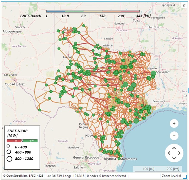
Texas Synthetic IPM Network Summary
| SAInt Object Type | Representative Object | Count |
|---|---|---|
| ENO | Nodes (Buses) | 6,717 |
| LI | Electric Lines | 7,173 |
| TRF | Transformers | 1,967 |
| SAInt Object Type | Generation Type | Capacity [GW] | Count |
|---|---|---|---|
| ESTR | Battery | 0.1 | 6 |
| PV | Solar | 2.3 | 36 |
| WIND | Wind | 0.41 | 152 |
| XGEN | Biomass | 0.1 | 2 |
| HGEN | Hydro | 0.5 | 22 |
| XGEN | Waste Heat | 0.2 | 8 |
| FGEN | Petroleum Coke | 0.1 | 2 |
| FGEN | Other Gases | 0.2 | 3 |
| FGEN | Internal Combustion | 0.5 | 45 |
| FGEN | Combustion Turbine | 6.9 | 127 |
| FGEN | Combined Cycle | 37.3 | 256 |
| FGEN | Steam Turbine | 11.8 | 45 |
| FGEN | Coal | 14.4 | 23 |
| FGEN | Nuclear | 5.0 | 4 |
| Name | FuelPriceDef [$MMBTU] | CO2 Emissions [g/MMBTU] | SO2 Emissions [g/MMBTU] | NOX Emissions [g/MMBTU] |
|---|---|---|---|---|
| Uranium | 0.5 | 0 | 0 | 0 |
| Natural Gas | 3.5 | 53454 | 0.272 | 16.68 |
| Coal | 2.0 | 95130 | 40.82 | 36.29 |
| Petroleum Coke | 7.5 | 102508 | 106.54 | 36.76 |
Ancillary Services
For the Texas Synthetic IPM market optimization, one ancillary service object (SAInt Object Type: ASVC) named “SPINNING_RESERVE” is included to represent an upward ramping reserve requirement. Generators in the following Groups have an associated ASVCX allowing them to contribute to the reserve requirement: Coal, Steam Turbine, Combined Cycle, Combustion Turbine, Internal Combustion, Petroleum Coke, and Other Gases.
Monitored Branches and Contingencies
For the Texas Synthetic IPM market optimization, 26 monitored branch objects (SAInt Object Type: MBR) are included. 21 of these are related to the contingency object (SAInt Object Type: CTG) named “DEFAULT”, indicating that thermal limits for these lines will be enforced for the N-0 network constrained case. The other 5 are defined as mon/con pair N-1 security constraints.
Scenarios for the Texas Synthetic IPM
ACPF_BASE_CASE
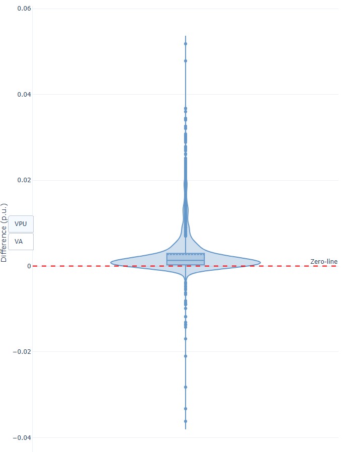
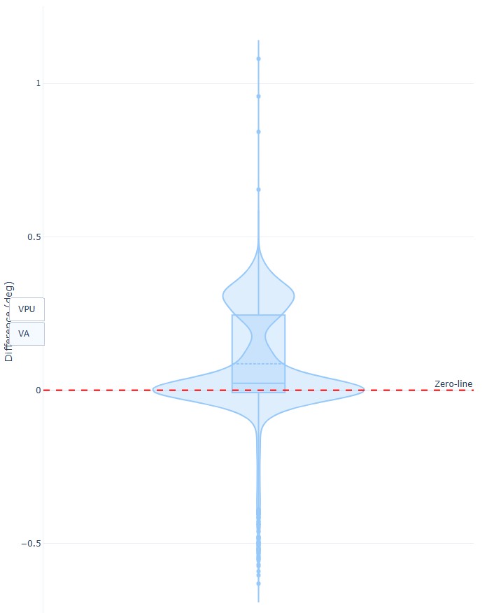
This scenario represents the base power flow case available from Texas A&M Electric Grid Test Case Repository. The ACPF solution for the ACPF_BASE_CASE was validated against the results reported in the original .RAW transmission planning case. Included here are the figures showing the difference between bus voltages and angles. To produce the full validation comparing the SAInt ACPF results with the .RAW, users can use the dot raw to saint plugin and translate the original .RAW file.
Voltage Angle Comparison with Original .RAW
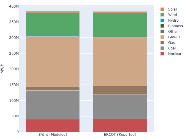
PCM_FULL_YEAR
This scenario represents the starting point for analysis using the Texas Synthetic IPM. It is an annual PCM scenario which uses the same network as the ACPF_BASE_CASE. This scenario is informed by market data posted by ERCOT and is intended to represent the 2019 operating year of ERCOT although it is not a technically rigorous representation of the ERCOT power market. Note that the solution file for this scenario is >20GB so it is not included in the .zip download for this dataset. Shown below is the annual generation comparison between the Texas Synthetic IPM annual PCM scenario and the actual generation reported by ERCOT for 2019.
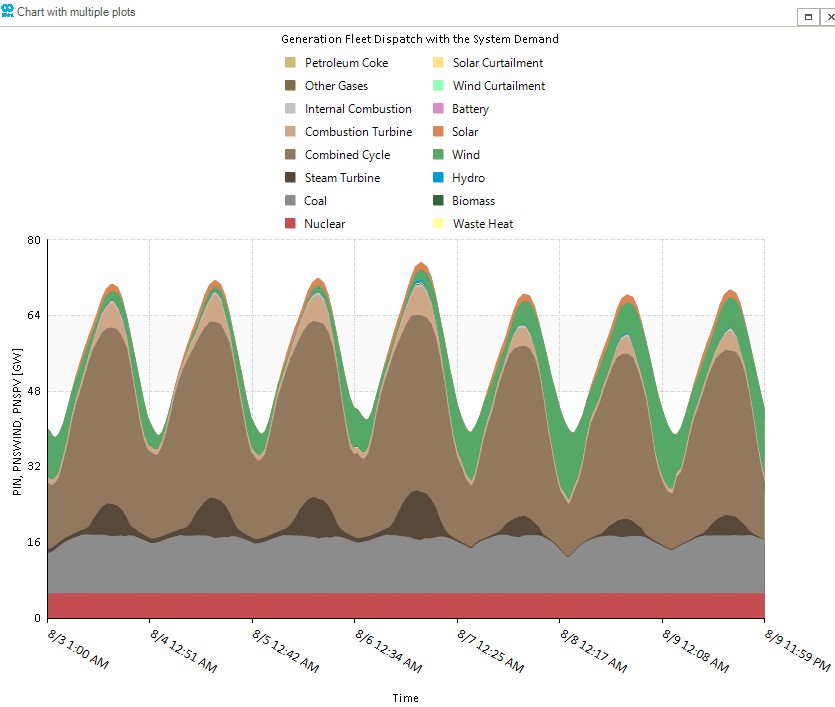
PCM_PEAK_WEEK
This scenario is the same as the PCM_FULL_YEAR except it includes representation of transmission losses and is only one week long. We include this scenario as an easy starting point for detailed analysis, although users can create any alternate scenario from either this or the annual scenario using the Integrated Planner.
PCM_PEAK_DAY
This is a one-day scenario without losses. It is intended to be a model for quick tests.