The Smart_Inverter network is a simplified distribution system that is configured with a single-phase smart inverter that exemplifies the various types of voltage support functionality that can be modeled in SAInt.
Download it here: Smart Inverters v25.5.16.zip (147.9 KB)
Overview
Smart inverters are distributed energy resources that are capable of providing voltage support via active and/or reactive power management based on the voltage at the point of interconnection. There are a few different types of common control mechanisms that constitute the smart inverter functionality including constant power factor, Volt-Var, and Volt-Watt. These control strategies can be easily implemented in SAInt using events with conditional expressions. This model shows off the implementation of smart inverter functionality with a single phase inverter, on a simplified distribution network.
Model
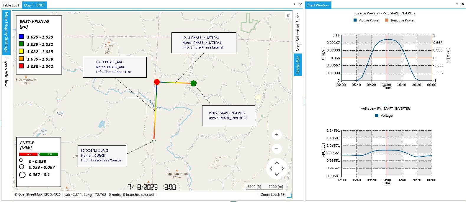
The model used to demonstrate the smart inverter functionality is a highly simplified distribution feeder circuit that shows a diverse loading throughout a 24 hour period. The model is an ideal source (representing the feeder head) connected to a single three-phase line with a downstream three-phase electric demand and solar object. A second line is a single-phase, that acts as the interconnection point for a second pv object, which is the inverter that is used to display the functionality. The Base_Case.esce scenario generates the active power output and resultant voltage shown in the model image presented above.
Constant Power Factor
The simplest type of reactive power support is to link the reactive power output to the active power output using a power factor (pf) setpoint. The mathematical relationship is the following:
where -
Note that the sign of the power factor is important; a negative pf will supply negative reactive power when positive active power is delivered.
The scenario Constant_Power_Factor.esce has the following property values relavant to the constant power factor control, with a single event generating the actual reactive power response.
| Attribute | SAInt Property | Value |
|---|---|---|
| Reactive Power Maximum (Q) | PV.SMART_INVERTER.QMAXDEF | 0.02 (Mvar) |
| Reactive Power Minimum (Q) | PV.SMART_INVERTER.QMINDEF | -0.02 (Mvar) |
| Constant Power Factor | PV.SMART_INVERTER.Constant | -0.95 |
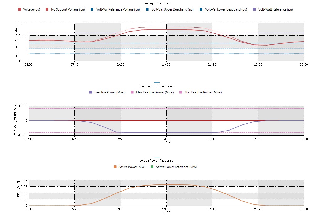
Executing the script inverter_response.ipy after the scenario is executed shows the reactive power response, and subsequent voltage impact, of the smart inverter:
Volt-Var
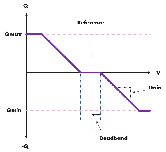
The Volt-Var control presents additional complexity in the reactive power response by applying a droop curve relationship between the point of interconnection voltage and the reactive power output of the inverter. The response is characterized by a reference voltage, a deadband, and a droop gain. The reactive power limits are still respected. The control is instanced with a single event. We encourage the modeler to investigate the properties used and how they link to the droop curve shown. The inverter_response.ipy script is your friend for viewing these results!
| Attribute | SAInt Property | Value |
|---|---|---|
| Reactive Power Maximum (Q) | PV.SMART_INVERTER.QMAXDEF | 0.02 (Mvar) |
| Reactive Power Minimum (Q) | PV.SMART_INVERTER.QMINDEF | -0.02 (Mvar) |
| Volt-Var Gain | PV.SMART_INVERTER.Constant2 | -10 |
| Volt-Var Reference | ENO.ENO_A.Constant | 1 |
| Volt-Var Deadband | ENO.ENO_A.Constant2 | 0.01 |
For Advanced Users: Because the Volt-Var control is referencing the voltage, which is a simulation result, the control must use the prior timestep voltage to generate the reactive power output. This is easily achieved in SAInt by using the etime property of objects in the conditional and value expressions of the events. If the power flow timestep is set at an hourly resolution, the previous hour solution will be used to calculate the reactive power of the current timestep. SAInt supports changing the timestep of a simulation with the TimeStep property. In the current model, this is reduced from 60 minutes to 15 minutes, so that the smart inverter has a few steps between updating the active power setpoints to arrive at a steady voltage/reactive power state. We recommend playing with the timestep, especially for larger inverters that have an appreciable impact on the system voltages!
Volt-Watt
Volt-Watt control simply reduces the active power maximum as a function of voltage. The maximum active power begins to be reduced for voltages exceeding the Volt-Watt Setpoint, and arrives at 0 at the Volt-Watt Cutoff. This control also relies on the previous timestep voltage values, and is therefore susceptible to some control oscillations. The scenario Volt_Watt.esce is set up with the following properties:
| Attribute | SAInt Property | Value |
|---|---|---|
| Reactive Power Maximum (Q) | PV.SMART_INVERTER.QMAXDEF | 0.02 (Mvar) |
| Reactive Power Minimum (Q) | PV.SMART_INVERTER.QMINDEF | -0.02 (Mvar) |
| Volt-Watt Cutoff | PV.SMART_INVERTER.Constant3 | 1.07 |
| Volt-Watt Setpoint | ENO.ENO_A.Constant3 | 1.03 |

The Volt-Watt control is implemented with a single event. Because this control only impacts the active power of the inverter, it can be used in conjunction with either constant power factor or Volt-Var control by activating the relevant event!
On/OFF Behavior
There is an additional event labeled On/Off Behavior that explicitly prevents the smart inverter from supplying reactive power unless there is a non-zero active power output. This can be easily turned off.
Note: the current network properties were chosen to highlight the interplay of the smart inverter functionality; i.e., as the active and reactive powers are changed in response to system voltages, the voltages will then change! If it is desired to remove this interplay, changed the CalcImp property of each line to False, which will establish two zero-impedance lines and allows the inverter to respond without impacting the voltages.