Overview
The Resource Adequacy plugin assesses the reliability of an electric power system to meet demand by simulating generator outages across multiple Monte Carlo draws. It uses probabilistic outage modeling to generate random availability scenarios for specified generators, runs each scenario through SAInt’s solver, and computes standard reliability metrics including Loss of Load Expectation (LOLE), Loss of Load Probability (LOLP), Loss of Load Hours (LOLH), and Expected Unserved Energy (EUE).
Versions Compatible with SAInt 3.8
- v0.1.7 (20.4 MB)
- v0.1.6
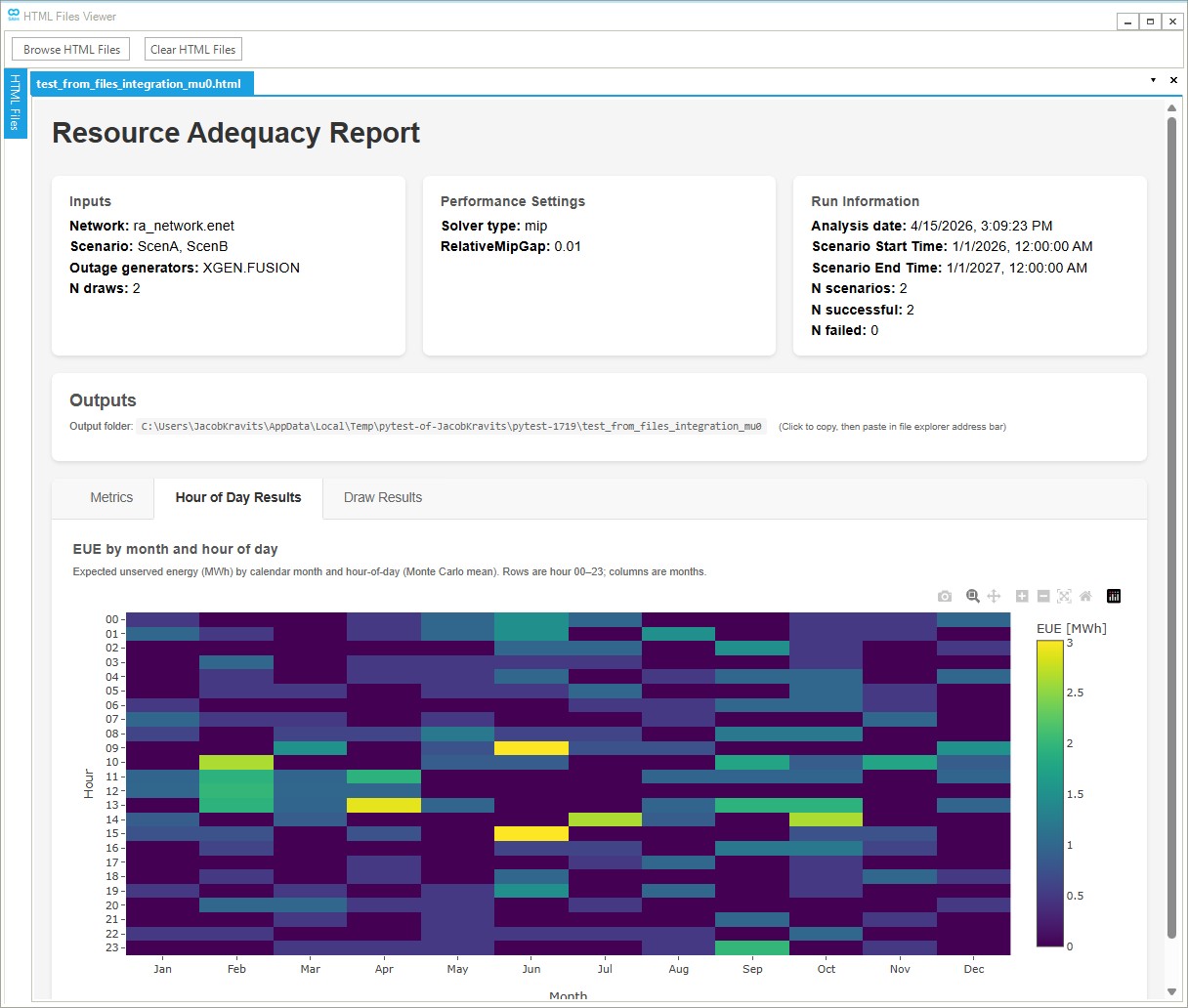
Screenshot:
Inputs
Required Files
SAInt Network File (.enet): The SAInt electric network file containing the network topology and components. If not specified explicitly, the plugin will look for a single .enet file in the same directory as the scenario file.
SAInt Scenario File (.esce): A SAInt DCUCOPF scenario file. The scenario must meet the following requirements:
| Requirement | Description |
|---|---|
| Scenario Type | DCUCOPF (DC Unit Commitment Optimal Power Flow) |
| Duration | 1 year (8760 hours for non-leap year, 8784 for leap year) |
| Time Resolution | Hourly (1-hour timesteps) |
| Optimization Horizon | Recommended: 1 day (24 hours) |
| Look-Ahead Period | Recommended: 1 hour |
| No Existing Outage Events | The scenario must not contain any pre-existing outage events for generators |
| No PREF Events | The scenario must not contain any PREF (active power reference) events for generators specified in the outage CSV |
Important: The plugin injects generator availability events via PREF profiles. If the scenario already contains PREF events for generators listed in the outage CSV, these will conflict with the plugin’s injected events and produce incorrect results.
Outage Specifications CSV (.csv): A CSV file defining the outage characteristics for each generator (or storage asset) to be modeled. See the Outage CSV Format section for details.
Optional Files
Multi-Scenario Configuration (YAML): A YAML file defining multiple scenarios to run with the same outage draws. This is commonly used to run resource adequacy across multiple weather years, where each weather year has its own demand profile scenario. When provided, the plugin runs each Monte Carlo outage draw across all scenarios (coupled runs), producing both per-scenario and weighted aggregate metrics.
Example scenarios.yaml for weather year analysis:
scenarios:
  - name: Weather2019
    path: demand_2019.esce
  - name: Weather2020
    path: demand_2020.esce
  - name: Weather2021
    path: demand_2021.esce
| Field | Type | Required | Description |
|---|---|---|---|
name |
string | Yes | Unique identifier for the scenario (e.g., weather year label) |
path |
string | Yes | Path to the .esce file (relative to the YAML file location) |
weighting |
float | No | Relative weight for aggregating metrics. If omitted for all scenarios, equal weights are used. If specified, must be positive and provided for all scenarios. |
When using multi-scenario mode:
- Paths in the YAML are resolved relative to the YAML file’s directory
- Scenario names must be unique within the configuration
- All scenarios must use the same network file
- The same outage draw is applied to each scenario, enabling consistent comparison across weather years
- Metrics are computed per-scenario and as weighted aggregates
Run Settings
Number of Draws: The number of coupled Monte Carlo base replications (outage scenarios) to simulate. More draws provide more statistically robust results but increase computation time. When using multi-scenario mode, the total number of ESIM executions equals n_draws × number of scenarios.
Performance Settings
Solver Type: The optimization solver to use for each draw:
- MIP (Mixed Integer Programming): Default; more accurate but slower, recommended for final results
- LP (Linear Programming): Faster, useful for screening and rapid iteration
Relative MIP gap: MIP optimality tolerance as a relative gap (default: 0.01). The solver stops when the gap between the best solution and the best bound is within this fraction. Lower values yield tighter solutions but longer run times.
Worker Processes: Number of parallel worker processes for executing draws. Increasing this value can significantly reduce total computation time on multi-core systems. Each worker runs draws independently. Recommended: set to the number of available CPU cores minus 1.
Note: The number of parallel workers is bounded by the number of licenses.
Save per-draw files (.enet, .esce, etc.): When set to Yes, the plugin saves a copy of the network and scenario files for each draw (e.g. per-draw .enet, .esce, .esol, .econ) in the output directory, useful for debugging or re-running individual draws. When No (default), only the aggregated results and report are written.
System Settings
Random seed: Random seed for draw generation; default 42. Same seed yields reproducible outage draws across runs.
SAInt API DLL Path: Path to the SAInt API DLL file. Default: C:\Program Files\encoord\SAInt-v3\SAInt-API.dll
Output Directory: The folder where the results will be saved. The plugin will:
- Copy the network and scenario files to this location
- Create a
draw_statessubdirectory containing individual draw results (and, if Save per-draw files is enabled, per-draw .enet and .esce files for each draw) - Generate a
results.jsonfile with all metrics and per-draw data - Generate an HTML report with visualizations
Logging Level: Controls the verbosity of logging output. Options: Debug, Info, Warning, Error, Critical
Outage CSV Format
The outage specifications CSV file defines which generators and storage assets should have stochastic forced outages modeled: forced outage rate, time to repair (in scenario timesteps), and must-run behavior.
Minimum up time and minimum down time are not specified in the CSV. For fuel generators (FGEN) and other non-XGEN types that expose them, MinUpTimeDef and MinDownTimeDef are read from the network (encoord electric objects reference §5.8). Values ≥ 3600 are interpreted as seconds (e.g. 14400 → 4 h at hourly resolution); smaller values as hours. They are converted to scenario timesteps using ENET.SCE.dt. Generic external generators (XGEN) do not expose those parameters (§5.6); the analysis uses 1 timestep each for minimum up and minimum down. The run fails if timesteps_to_repair is less than the minimum down time in timesteps.
Do not include legacy columns min_up_time or min_down_time in the CSV; they are rejected.
| Column | Type | Required | Description |
|---|---|---|---|
generator_id |
string | Yes | The SAInt generator or storage object ID (e.g., FGEN.SIMONDS, XGEN.FUSION, STOR.BATTERY1) |
outage_rate_fraction |
float | Yes | Forced Outage Rate (FOR) as a fraction between 0 and 1 (e.g., 0.05 for 5%) |
timesteps_to_repair |
integer | Yes | Time to Repair (TTR) — consecutive timesteps the asset remains unavailable per outage (same time resolution as the scenario, e.g. hours for hourly scenarios). Must be ≥ minimum down time in timesteps (from MinDownTimeDef when readable, or 1 for XGEN). |
must_run_status |
boolean | Yes | If true, asset uses ONOFF constraint when available; if false, uses ON constraint |
Example Outage Specifications
Typical forced outage parameters (minimum up/down come from the network for FGEN/STOR, or XGEN defaults, not the CSV):
| Asset | Asset Type | Forced Outage Rate (%) | Time to Repair (timesteps) | Must Run |
|---|---|---|---|---|
| FGEN.SIMONDS | Gas Turbine | 10% | 24 | No |
| FGEN.DARTMOUTH | Gas Turbine | 10% | 24 | No |
| XGEN.FUSION | External Generator | 2.5% | 1 | Yes |
Example Outage CSV
generator_id,outage_rate_fraction,timesteps_to_repair,must_run_status
FGEN.SIMONDS,0.1,24,false
FGEN.DARTMOUTH,0.1,24,false
XGEN.FUSION,0.025,1,true
This example configures two gas turbine generators with 10% forced outage rate and 24 timesteps repair time, plus an external generator with 2.5% outage rate and 1 timestep repair time. Minimum up/down constraints for FGEN assets are read from the .enet file; XGEN uses 1 timestep for both.
Column Details
generator_id: Must match the exact SAInt object identifier including the prefix:
FGEN.for fuel generatorsXGEN.for generic external generators
outage_rate_fraction (Forced Outage Rate): The probability that a forced outage event begins at any given hour. This represents the Forced Outage Rate (FOR) commonly used in reliability studies. A value of 0.1 means there is a 10% chance per hour that the asset will experience a forced outage (subject to repair time and constraint requirements).
Note: With the generator constraints (i.e timesteps_to_repair, minimum down/up times), the draw generator might not produce tge exact value of the outage fraction specified in the outage csv file. It will generate an outage fraction with 1 e-4 tolerance from the specified fraction.
Typical forced outage rates by technology:
- Nuclear: 2-5%
- Coal: 5-10%
- Combined Cycle Gas: 3-6%
- Simple Cycle Gas Turbine: 5-12%
- Wind: 2-5%
- Solar PV: 1-3%
- Battery Storage: 1-3%
timesteps_to_repair (Time to Repair): Once a forced outage begins, the asset remains unavailable for this many consecutive hours. This represents the Time to Repair (TTR) or Mean Time to Repair (MTTR).
Typical repair times by technology:
- Nuclear: 72-168 hours (3-7 days)
- Coal: 24-72 hours (1-3 days)
- Combined Cycle Gas: 12-48 hours
- Simple Cycle Gas Turbine: 8-24 hours
- Battery Storage: 4-24 hours
must_run_status: Controls the SAInt event parameter used when the asset is available:
trueor1: UsesONOFFparameter (asset must run when available)falseor0: UsesONparameter (asset can run when available)
Generator MinUpTimeDef / MinDownTimeDef (network, non-XGEN): After the network is loaded, the plugin reads these where the object type supports them and converts them to timesteps (seconds if ≥ 3600, else hours). XGEN uses 1 timestep each for min up/down (no network read). The draw generator then enforces:
- Minimum up: After each outage ends, the asset remains available for at least that many consecutive timesteps before the next outage can begin (including after the last outage in the horizon).
- Minimum down: Each outage block lasts
max(timesteps_to_repair, min_down_timesteps); the plugin requirestimesteps_to_repair >= min_down_timestepsso the repair time is never shorter than the network minimum down time.
Computation Logic
The resource adequacy assessment follows these steps:
1. Parse Inputs and Initialize
The plugin:
- Loads the network and scenario files into SAInt
- Parses the outage CSV to extract generator outage specifications
- If a multi-scenario YAML config is provided, parses scenario list and weights
- Enriches each generator’s min up/down (network for FGEN/STOR, 1/1 timesteps for XGEN) and validates repair time vs. minimum down time
- Creates the output directory structure
- Extracts scenario time information (start time, end time, timestep duration)
2. Generate Monte Carlo Draws
For each base replication (draw), the plugin generates a random availability schedule for each generator:
- Binary Sampling: For each generator, generates a binary array (0 = unavailable, 1 = available) for all timesteps using constrained random sampling
- Outage Rate: The sampling respects the specified
outage_rate_fractionas the target probability of being in an outage state - Repair Time: Each outage lasts
max(timesteps_to_repair, min_down_timesteps)consecutive unavailable timesteps, withmin_down_timestepsfromMinDownTimeDefwhen available (or 1 for XGEN);timesteps_to_repairmust be at least that value. - Minimum Up Time: After each outage the generator stays available for at least
min_up_timestepsconsecutive timesteps (including the period after the last outage in the horizon).
In multi-scenario mode (e.g., weather year analysis), each base replication generates one outage schedule that is applied identically across all scenarios (coupled draws). This ensures consistent comparison across weather years for the same outage realization.
3. Execute Draws
Each draw is executed through SAInt:
- Inject Events: The availability schedule is converted to SAInt events that modify generator availability profiles
- Run Simulation: SAInt runs the scenario with the modified generator availabilities
- Collect Results: Load shedding data is extracted from the simulation results
- Parallel Execution: If
worker_processes > 1, multiple draws are executed in parallel
In multi-scenario mode, total ESIM executions = n_draws × number of scenarios.
4. Compute Metrics
After all draws complete, the plugin aggregates results into standard reliability metrics:
Annual Metrics:
- LOLE (Loss of Load Expectation): Expected number of days per year with load shedding
- LOLP (Loss of Load Probability): Probability that load shedding occurs in any given period
- LOLH (Loss of Load Hours): Expected number of hours per year with load shedding
- EUE (Expected Unserved Energy): Expected total energy not served (MWh)
- Mean Load Shedding Events: Average number of distinct load-shedding event blocks per draw
- Mean Peak Power Not Served: Average of peak |PNS| (MW) across draws
- Mean Max Event Unserved Energy: Average of the largest single event’s unserved energy (MWh) across draws
Temporal Breakdowns:
- Monthly metrics (keyed by
YYYY-MM) - Daily metrics (keyed by
YYYY-MM-DD) - Hourly metrics (keyed by
YYYY-MM-DD HH:00) - Month-hour metrics (keyed by
MM-HHfor calendar month and hour-of-day patterns) - Seasonal metrics (keyed by
YYYY-Seasonusing Northern Hemisphere meteorological seasons: Spring Mar-May, Summer Jun-Aug, Fall Sep-Nov, Winter Dec-Feb)
Per-Draw Metrics:
- Individual draw success/failure status
- Per-draw total unserved energy (MWh)
- Maximum hourly unserved energy (MWh)
- Maximum load shedding event energy (MWh) and power (MW)
- Number of load shedding events
Multi-Scenario Aggregation (e.g., weather years):
When multiple scenarios are configured:
- Per-scenario metrics: Full metric breakdowns computed for each weather year/scenario independently
- Weighted metrics: Headline aggregate metrics weighted by scenario weights (equal weights if not specified)
5. Generate Outputs
The plugin produces:
results.json: Complete metrics data in JSON format- HTML report: Interactive visualization of results with EUE heatmaps and per-draw tables
Output
The plugin generates the following outputs in the specified output directory:
1. HTML Report (<output_folder_name>.html)
An interactive HTML report containing:
- Summary statistics and key metrics table
- EUE heatmap by month and hour-of-day
- Per-draw status table with load-shedding statistics
- Per-scenario and weighted metric breakdowns (when using multi-scenario/weather year mode)
2. Results JSON (results.json)
A JSON file containing complete analysis data including metadata, all metrics (per-draw, per-scenario, weighted), and detailed draw results. Useful for programmatic post-processing or integration with other tools.
3. Draw States Directory (draw_states/)
Contains individual draw result files for debugging and detailed analysis. If Save per-draw files is enabled in Performance Settings, this directory also includes per-draw network (.enet), scenario (.esce), solution (.esol), and convergence (.econ) files for each Monte Carlo draw.
4. Copied Network and Scenario Files
The original network (.enet) and scenario (.esce) files are copied to the output directory for reference and reproducibility.
Interpreting Results
Key Metrics
LOLE (Loss of Load Expectation): The expected number of days per analysis period when demand exceeds available supply. Industry standards often target LOLE < 0.1 days/year (1 day in 10 years). Computed as the mean across draws of distinct calendar days with at least one hour of load shedding (NERC-style day count).
LOLP (Loss of Load Probability): The probability of experiencing a loss of load event in any given period. Expressed as a fraction (0.01 = 1% probability). Computed as the mean across draws of the ratio (hours with shedding / total hours).
LOLH (Loss of Load Hours): The expected number of hours per analysis period with unserved load. Provides more granular insight than LOLE.
EUE (Expected Unserved Energy): The expected total energy (MWh) that cannot be served due to supply shortfalls. Useful for economic analysis of reliability costs.
Mean Load Shedding Events: The average number of distinct contiguous load-shedding event blocks per draw. An “event” is a sequence of consecutive hours with non-zero power not served.
Mean Peak Power Not Served (MW): The average across draws of the maximum hourly power shortfall (|PNS|) in MW.
Mean Max Event Unserved Energy (MWh): The average across draws of the largest single load-shedding event’s total energy shortfall.
Temporal Breakdown Keys
- Monthly:
YYYY-MM(e.g.,2024-07) - Daily:
YYYY-MM-DD(e.g.,2024-07-15) - Hourly:
YYYY-MM-DD HH:00(e.g.,2024-07-15 14:00) - Month-Hour:
MM-HH(e.g.,07-14for July at 2 PM) — useful for identifying diurnal/seasonal patterns - Seasonal:
YYYY-Seasonusing Northern Hemisphere meteorological seasons:- Spring: March–May
- Summer: June–August
- Fall: September–November
- Winter: December–February (December of year Y maps to
(Y+1)-Winter)
Changelog
v0.1.6
- Updated solver defaults.
v0.1.6
- Multi-scenario support: YAML configuration for running multiple weather years or demand scenarios with coupled outage draws
- Scenario weighting: Optional weights for computing weighted aggregate metrics across weather years/scenarios
- Enhanced metrics structure:
metrics.by_scenario: Per-scenario metric breakdownsmetrics.weighted: Headline weighted aggregate (or single-scenario metrics when only one scenario)metrics.by_draw: Per-draw statistics including event counts and peak values
- New temporal breakdowns:
- Month-hour metrics (
MM-HH) for diurnal/seasonal pattern analysis - Seasonal metrics using Northern Hemisphere meteorological seasons
- Month-hour metrics (
- New per-period metrics:
- Mean load shedding events
- Mean peak power not served (MW)
- Mean max event unserved energy (MWh)
- HTML report improvements:
- EUE heatmap by month and hour-of-day
- Per-draw status table with detailed statistics
- Multi-scenario metric tables
- STOR (storage) asset support in outage CSV
- MIP solver is the default (LP optional for faster screening)
- Save per-draw files now includes .esol and .econ files
- Network path auto-discovery when single .enet file exists in scenario directory
- Monte Carlo draw generation with constrained binary sampling
- Support for generator outage specifications via CSV
- Configurable outage rate, repair time, and must-run status per generator
- Minimum up/down from
MinUpTimeDef/MinDownTimeDeffor non-XGEN types, fixed 1/1 timesteps for XGEN, with validation (timesteps_to_repair≥ minimum down) - Optional script
scripts/saint_smoke_run.pyfor a minimal load → one draw →runESIMcheck - Parallel draw execution with configurable worker processes
- Comprehensive reliability metrics (LOLE, LOLP, LOLH, EUE)
- Temporal breakdowns (annual, monthly, daily, hourly)
- Per-draw metrics and statistics
- HTML report generation with visualizations
- JSON results output for programmatic access