The GNET95 network is a synthetic database derived from publicly available data provided by the US Energy Information Administration (EIA) in the US Energy Atlas Natural Gas Infrastructure and Resources. The MRD matches the area covered by the ENET39, including the New England region and its connections to Canada and New York State.
Download it here: GNET95 v2025.09.zip (567MB)
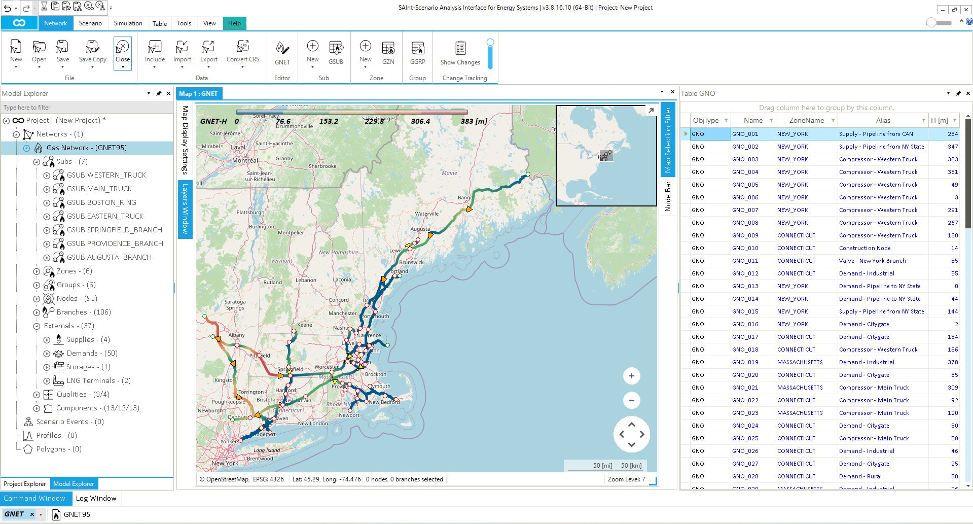
Figure 1: GNET95 topology and nodal elevation
Disclaimer
The GNET95 dataset is an illustrative representation of part of the US natural gas system. It is not a technically rigorous reproduction of the actual infrastructure. The names of the supply and demand points are purely suggestive. Pipeline and compressor sizing, pressure limits, and flow capacities are designed for demonstration and analysis purposes. The network layout is a simplified topology based on the US Energy Atlas, retaining the main trunk lines and branches supplying gas to the region.
This MRD was developed by encoord GmbH for the Scenario Analysis Interface for Energy Systems (SAInt) planning software, which is provided “as is” at no cost. encoord GmbH disclaims all responsibility for its use by others and makes no warranties, express or implied, regarding its quality, reliability, safety, or suitability. encoord GmbH will not be liable for any direct, indirect, or consequential damages related to its use.
License
This work is licensed under “Creative Commons Attribution-NonCommercial-ShareAlike 4.0 International” (CC BY-NC-SA 4.0) by the creator encoord GmbH. To view a copy of this license, visit https://creativecommons.org/licenses/by-nc-sa/4.0/.
This license requires that reusers give credit to the creator. It allows reusers to distribute, remix, adapt, and build upon the material in any medium or format, for noncommercial purposes only. If others modify or adapt the material, they must license the modified material under identical terms. It is stipulated that:
- BY: Credit must be given to you, the creator.
- NC: Only noncommercial use of your work is permitted. Noncommercial means not primarily intended for or directed towards commercial advantage or monetary compensation.
- SA: Adaptations must be shared under the same terms.
Overview
The GNET95 network is a simplified representation of the natural gas pipeline infrastructure in the New England region, derived from the US EIA’s Energy Atlas. This region was selected to align with the ENET39 MRD. The network is divided into seven subsystems (SAInt Object Type: GSUB), each representing a distinct section of the overall system. It includes three high-pressure pipeline trunks that transport gas from supply points to demand centers. In addition, there are four low-pressure subsystems, including a ring around the Boston area and three branches that deliver gas to end users. The network is also divided into six zones (SAInt object type: GZN), each representing a different state in the New England region. Table 1 below provides an overview of the objects that form the GNET95 MRD.
| SAInt Object Type | Description | Count |
|---|---|---|
| GNO | Nodes | 95 |
| GPI | Pipes | 88 |
| GCS | Compressor Stations | 9 |
| GCV | Control Valves | 7 |
| GVA | Valve | 1 |
| GSUP | Gas Supply | 4 |
| GDEM | Gas Demand | 50 |
| GSTR | Underground Storage | 1 |
| LNG | LNG Terminal | 2 |
Developing the GNET95 Network: From topological pipeline data to synthetic dataset
In SAInt, a network is a directed graph comprising of objects such as nodes, branches, and externals. Each network is characterized by its geometric, topological, relational, and static properties of all its objects. The GNET95 network is a synthetic representation of the New England gas infrastructure with some additional modifications. The sections below explain the key network parameters and design assumptions used to create the MRD.
Network Topology
The topology data were collected from the EIA’s Energy Atlas, which represents both intrastate and interstate pipelines in the New England region. The original database contained approximately 2,400 individual pipeline segments. After reviewing the available data, the primary gas infrastructure was identified and the topology simplified by combining smaller pipeline segments into longer continuous routes and removing short terminal branches that ended at a single node without further connectivity. The final topology was then adjusted to align with the ENET39 MRD.
The resulting dataset includes 95 individual nodes (SAInt Object Type: GNO), representing supply points, storage facilities, demand centers, and construction nodes connected to compressor stations, control valves, valves, and pipeline segments.
For each node, elevation data (in meters) was obtained from NASA’s Shuttle Radar Topography Mission (SRTM), which used radar measurements from space to create one of the most detailed digital elevation models of the Earth. Elevations were assigned based on the latitude and longitude coordinates of each node. Pipeline lengths were calculated using the built-in geometric length calculator in SAInt. The network is divided into zones and subsystems. Each zone (SAInt Object Type: GZN) represents the US states through which the network topology passes. In comparison, each subsystem (SAInt Object Type: GSUB) represents a distinct section of the pipeline system. The subsystems are:
- WESTERN_TRUCK: Transports gas from the Ontario (Canada) interconnection and Northern NY State wellsites to the primary demand hub in New York City and Long Island.
- MAIN_TRUCK: Connects the Western Trunk and NY State pipeline system to the low-pressure branch subsystems (Springfield, Providence, and the Boston Ring).
- EASTERN_TRUCK: Transports gas from the New Brunswick (Canada) interconnection and the Portland LNG terminal to the Boston Ring.
- BOSTON_RING: Encircles the Boston metropolitan area, delivering gas to urban and residential end users. It also connects to an underground storage facility and an LNG terminal.
- SPRINGFIELD_BRANCH: Supplies gas to urban, industrial, and power plant end users in the Springfield area.
- PROVIDENCE_BRANCH: Supplies gas to major industrial and power plant users in the Providence area.
- AGUSTA_BRANCH: Supplies gas to rural areas and power plants around Augusta.
The trunk subsystems act as “gas highways” transporting large volumes of gas at higher pressures (50–85 [bar-g]) from supply points to major demand hubs such as New York City and Boston. In contrast, the Boston Ring and branch subsystems function more like “local streets and avenues,” distributing gas at lower pressures (5–40 [bar-g]) to supply end users, including city gates, industrial facilities, power plants, and rural areas.
Gas Demand
The gas demand (SAInt Object Type: GDEM) data for the GNET95 network was developed using a structured methodology that combines demand classification, peak demand estimation, and load profile shaping based on climatological patterns. The process ensures that demand profiles reflect both seasonal and hourly variations consistent with observed regional energy use in the northeastern United States. Each demand in the network was defined to represent a specific type of end user:
- Citygate: large metropolitan centers with residential and commercial loads, dominated by space-heating.
- Industrial: locations with heavy manufacturing or concentrated industrial activity.
- Power Plants: gas-fired generators and turbines consuming fuel for electricity production.
- Rural: smaller towns and agricultural communities with lower and more seasonal demand.
Table 2 shows how these demand nodes were classified and grouped into gas groups (SAInt Object Type: GGRP). Each group aggregates demand nodes of a similar type, providing a simplified representation for analysis. The table also summarizes the number of demand nodes in each group, the total aggregated maximum flow (SAInt Object Parameter: QMAX), the minimum delivery pressure (SAInt Object Parameter: PMIN) required before demand is curtailed to maintain network pressure limits, and the operational control settings applied when running different scenarios.
| SAInt Group | Gas Demand Description | Count | Max Flow [ksm3/h] | Min Pressure, [bar-g] | Operational Control |
|---|---|---|---|---|---|
| NYC | New York City & Long Insland | 2 | 3,363 | 5 | Flow Set Point (QSET) |
| BOS | Boston | 10 | 390 | 5 | Flow Set Point (QSET) |
| CGS | Citygate Stations | 13 | 346 | 5 | Flow Set Point (QSET) |
| RUR | Rural & Agricultural | 5 | 107 | 5 | Flow Set Point (QSET) |
| IND | Industrial Facilities | 15 | 644 | 20 | Flow Set Point (QSET) |
| GFG | Power Plants & Electric Production | 5 | 737 | 25 | Flow Set Point (QSET) |
NOTE
Main demand points, New York City, Long Island, and Boston, are grouped separately. New York City and Long Island are modeled as the downstream interstate interconnection with the broader US gas infrastructure. However, due to their urban characteristics, they are modeled as city gate demand.
Peak Demand Estimation
Estimating peak demand (SAInt Object Parameter: QMAXDEF) is essential for creating accurate demand representations for the GNET95 network. Each end-user has distinct consumption behaviors, which require individual methodologies and adjustments to estimate their peak. This ensures that demand values capture both technical characteristics, such as power plant generator capacity, and regional demand drivers, including heating requirements in colder climates.
Power Plant Demand
For demand associated with power plants, peak gas requirements were derived from the operational characteristics of the generation fleet. Each power plant’s gas demand reflects a fuel object (SAInt Object Type: FUEL) linked to a fuel generator (SAInt Object Type: FGEN) in the ENET39 dataset. The generator’s nominal capacity (SAInt Object Parameter: PMAX) and fuel consumption coefficients (SAInt Object Parameters: FCO, FC1, and FC2) are used to estimate the maximum gas required to operate at full capacity.
NOTE
In future MRDs, these objects will be integrated through SAInt’s Hub Systems (SAInt Object Type: HUBS) and other methods, which serve as coupling points between the electric and gas networks. This approach will enable the creation of combined network models to analyze interactions between electricity and gas systems and support coordinated planning across both infrastructures.
City Gate, Industrial and Rural Demand
For other demand types, peak demand was determined using a classification-based methodology that captures how gas is consumed in cities, industrial hubs, and rural areas.
- Each demand node was geographically placed near a representative city or point of interest. Cities were then classified based on their dominant demand characteristics into city gate (urban/residential), industrial facilities, or rural/ agricultural areas.
- Industry practice and ISO filings were used to assign baseline Peak-to-Average Ratios (PAR) values to each classification. For city gate, industrial, and rural areas, the PAR values are typically around 3.2, 1.2, and 3.5. These ratios represent how much higher peak demand is relative to the annual average, reflecting differences in load variability.
- The annual average demand for each city was estimated using population data, regional energy consumption benchmarks, and end-use gas intensity factors. This value served as the baseline against which peaks were scaled.
- Peak loads were then tuned to reflect weather sensitivity, using correlations with heating degree days (HDDs) to capture the impact of cold weather on heating-driven demand. Colder regions and winter periods, therefore, show proportionally higher demand.
- For cities or regions with significant industrial activity, industrial adders were applied. These reflect continuous, process-driven demand that remains largely independent of seasonal heating needs.
The final peak demand values [ksm³/h] were obtained by scaling the annual average with the appropriate PAR factor and refining the result with HDD adjustments and industrial adders. This produced demand estimates that are both data-driven and climate-sensitive, ensuring that peaks align with observed patterns in the New England region.
Annual Demand Profile
The development of annual demand profiles ensures that demand in the GNET95 network reflects both seasonal variations and hourly fluctuations consistent with observed energy consumption patterns in the region. After peak demand values were established for each node, demand profiles were constructed to capture climatological effects, intra-day cycles, and realistic year-round variability.
Power Plant Demand
The demand associated with power plants is directly linked to the gas-fired generation fleet dispatch from ENET39, using the outputs of the PCM_FULL_YEAR scenario to optimize the dispatch under market conditions. This ensures that gas demand at power plants reflects electricity market outcomes, operational constraints, and generator fuel consumption, maintaining consistency between the gas and electricity networks. GNET95 includes individual demand data for each generator off-take point.
NOTE
In future MRDs, we will explore methods to better coordinate power market operations with gas network operations through an integrated workflow. This will allow us to assess how factors such as generation mix, carbon pricing, and market mechanisms influence gas demand and network operation. In turn, incorporating gas operational constraints (e.g., pipeline capacity or pressure limits) into electricity market redispatch will enable identification and mitigation of bottlenecks and downstream effects across both infrastructures. Ultimately, this iterative approach will support coordinated planning of gas and electricity systems and improve resilience under different policy and market conditions.
City Gate, Industrial and Rural Demand
For demand categories associated with city gate, industrial, and rural nodes, normalized annual demand curves were developed using a structured stepwise approach:
- Demand was distributed across weeks using long-term climatological temperature averages. Winter months (Dec–Feb) exhibited high baselines driven by heating loads, summer months (Jun–Aug) reflected minimal non-heating demand, and spring/fall periods represented transitional shoulder seasons.
- Typical intra-day load profiles were applied to represent realistic daily cycles:
- City gate (urban/residential): strong morning and evening peaks reflecting residential heating and household activity.
- Industrial: flatter profiles with relatively constant demand across the day.
- Rural: similar to city gate patterns but with more pronounced seasonal swings.
- For each season, representative weeks were constructed using the intra-day load shapes, with modifications applied for weekends and month-to-month differences. This step ensured variability and realism at the weekly level.
- Weekly and seasonal variability was introduced based on historical climatological averages to capture realistic fluctuations. To prevent discontinuities, interpolation and neighbor-week averaging were applied, ensuring smooth transitions between weeks and seasons.
- Each profile was normalized so that the annual average equaled 1.0, with PAR values re-applied to ensure consistency with peak demand calculations.
- The final profiles were extended across 8,760 hours, producing complete normalized annual demand curves. These curves were then scaled to the city-level demand estimates derived from population, energy consumption benchmarks, and intensity factors.
Gas Supply, LNG Terminals, and Underground Storage
The gas supply points (SAInt Object Type: GSUP), LNG terminals (SAInt Object Type: LNG), and underground storage (SAInt Object Type: GSTR) in the GNET95 network were defined to represent realistic natural gas sources for the New England region. Their capacities and operation constraints were derived from a combination of cross-border pipeline interconnection data, regional gas infrastructure, storage facilities, and wellsite estimates, based on publicly available information from the EIA’s Energy Atlas – Natural Gas Infrastructure and Resources. This ensures that modeled inflows and storage operations reflect plausible infrastructure conditions.
Cross-Border Interconnection
Supply capacities at the Canadian and New York State interconnections were derived from published cross-border transfer limits and adjusted to align with the GNET95 network demand. These interconnections represent the primary inflows of natural gas into the system. The Canadian interconnections operate under flow control set points (SAInt Event Parameter: PSET), helping to stabilize pressure on the western side of the network, where the largest demand hub (NEW_YORK and LONG_ISLAND) is located.
Table 3 summarizes the cross-border interconnections, including maximum transfer capacity, operational controls, and gas quality. For all supply points, the maximum flow (SAInt Object Parameter: QMAXDEF) is defined by the technical maximum flow of the connected pipeline, rather than an assumed operational maximum. The operational pressure range of each supply point is between 50 and 80 [bar-g].
| SAInt Group | Supply Name | Gas Supply Description | Transfer Volume, [ksm3/h] | Operational Control | Gas Quality (GCV, [MJ/sm3]) |
|---|---|---|---|---|---|
| SUP_CAN | WADDINGTON | National Cross-Border Canada Waddington, Ontario |
1,356 | QSET | CANADA (39.438) |
| SUP_CAN | SAINT_JOHN | National Cross-Border Canada Saint John, New Brunswick |
980 | QSET | CANADA (39.438) |
| SUP_US | SCHENECTADY | Interstate Cross-Border Northern New York State |
1,794 | PSET | DEFAULT (37.344) |
| SUP_US | NEWBURGH | Interstate Cross-Border Central New York State |
1,500 | PSET | DEFAULT (37.344) |
TIP
SAInt’s gas hydraulic solver always attempts to respect the user’s operational controls. However, the solver will search for feasible solutions within bounds defined by system constraints. If necessary, it adjusts control parameters or relaxes constraints by applying a penalty price (PRC). Constraints with higher penalty prices are prioritized. If a constraint has a penalty set to infinity, it is considered a hard constraint that cannot be violated. See the SAInt documentation for additional details.
LNG Terminal
The LNG terminals (SAInt Object Type: LNG) are synthetic facilities modeled after real infrastructure in other regions of the US, but scaled down to match the reduced scope of the GNET95 dataset. This scaling maintains LNG’s strategic role as a secondary supply source while keeping capacities consistent with the model. Both terminals are located along the eastern coast and operate under flow control set points (SAInt Event Parameter: QSET). Table 4 provides a summary of the operational characteristics, including maximum inventory (SAInt Object Parameter: INVMAX), maximum vessel size (SAInt Object Parameter: VESMAX), maximum flow rates (SAInt Object Parameter: QMAX), and gas quality of each terminal.
| SAInt Group | Terminal Name | LNG Terminal Description | Inventory Size, [Msm3] | Max Vessel Size, [m3] | Max Flow, [ksm3/h] | Gas Quality (GCV, [MJ/sm3]) |
|---|---|---|---|---|---|---|
| SUP_LNG | STELLWAGEN | Boston LNG terminal Seasonal supply contract |
113 | 160,000 | 472 | LNG (41.358) |
| SUP_LNG | SOUTH_PORTLAND | Portand LNG terminal Fixed supply contract |
127 | 160,000 | 530 | LNG (41.358) |
The STELLWAGEN terminal provides a seasonal supply to the BOSTON_RING, operating based on a threshold demand level. During periods of peak demand above this threshold, the terminal operates at full capacity to inject regasified gas into the network. During lower-demand periods, the facility reduces production to only one supply train. The SOUTH_PORTLAND terminal, connected to the EASTERN_TRUCK, functions as a backup supply source under a fixed supply contract. Both terminals receive LNG vessel deliveries approximately every 30 days.
Underground Storage
The underground storage facility (SAInt Object Type: GSTR) is also a synthetic facility, scaled from existing infrastructure in other US regions to fit the GNET95 dataset. The CHELSEA storage facility, connected to the BOSTON_RING, is designed to support the metropolitan area by maintaining pressure levels and ensuring continuous service for end users. The facility operates under a pressure control set points (SAInt Event Parameter: PSET) with a working inventory (SAInt Object Parameter: INVMAX) of 152 [Msm3] and operational envelope defined by the injection and withdrawal limits of the facility.
TIP
Refer to the How-to Guide Define Properties of a Gas Storage in the SAInt documentation for a refresher on the different properties used to define gas storage facilities and their operational envelopes.
Pipe and Valve Sizing
The GNET95 network includes 88 individual pipelines (SAInt Object Type: GPI). The sizing of each segment was determined based on the estimated flow through the segment, with an additional design factor to ensure safety and provide operational headroom. The pipe specifications such as the diameter (SAInt Object Parameter: D) and wall thickness (SAInt Object Parameter: WTH) were assigned according to standard sizing guidelines from ASME/ANSI B36.10M and API 5L. Sizing ranges from NPS12 (DN300) to NPS48 (DN1200) depending on the calculated flow, with wall thickness designation XS. Other pipeline specification such as roughness (SAInt Object Parameter: RO), efficiency (SAInt Object Parameter: Eff), and heat transfer coefficient (SAInt Object Parameter: HTC) are fixed for all pipeline segments. The pipeline lengths (SAInt Object Parameter: L) are set to match the geographical length (SAInt Object Parameter: LGEO) calculated by SAInt using map coordinates. This ensures that bends and routing are accounted for. The only exception is for segments connected to valves or compressor stations, where the additional facility length is included.
The network also includes seven control valves (SAInt Object Type: GCV), which separate the high-pressure trunks from the lower-pressure branches and the Boston Ring. These valves reduce pressure to 40 [bar-g] and operate within a control range of 5 and 85 [bar-g]. Maximum flow (SAInt Object Parameter: QMAXDEF) based on pipeline connection. One additional valve (SAInt Object Type: GVA) is included to emulate supply disruptions to the NEW_YORK demand. Both valve types are sized according to their downstream pipeline connections.
Compressor Station
The GNET95 includes nine different compressor stations, strategically located along the high-pressure trunks to maintain operating pressures. The compressor stations are spaced approximately 100–150 km apart and operate at around 70 [bar-g] to maintain trunk pressures without exceeding the network’s maximum operating pressure of 85 [bar-g]. Each station has an operational range of 50 and 85 [bar-g] and flow limits determined by the upstream pipeline connections. The maximum pressure ratio (SAInt Object Parameter: PRMAXDEF), driver power (SAInt Object Parameter: POWDMAXDEF), and shaft power (SAInt Object Parameter: POWSMAXDEF) are based on peak system demand conditions with added safety factors. Compressors are modeled with fuel extraction, meaning they consume a portion of the transported gas to operate.
NOTE
Compressor stations are modeled using adiabatic efficiency (SAInt Object Parameter:EFFHDEF) and mechanical efficiency (SAInt Object Parameter:EFFMDEF), both of which can be varied over time or under different system conditions. Using conditional events, SAInt allows simulation of operational scenarios such as ambient temperature effects or driver power loading. Future MRDs will also explore the design of electric-driven compressors, coupling gas compression with electricity demand to enable cross-sector system analysis.
Modeling Scenarios with GNET95
In SAInt, a scenario represents a specific case study applied to a network. A gas hydraulic simulation scenario is defined by its type (e.g., SteadyGas or DynamicGas), a time window (from StartTime to EndTime), and a time step. It may also include a set of events and profiles. An event represents a change in settings, controls, or constraints of an object at a specific point in time during the scenario’s execution. A profile is a sequence of equidistant data points that includes information on how these data points are processed in terms of time step, interpolation, sampling, and periodicity. Profiles can be assigned to events to control how their values evolve.
Tip
Scenario profiles can be viewed through the SAInt GUI by navigating to the Scenario Tab and selecting the [EPRF] button, after loading the network and scenario files. To explore the list of events that are part of a scenario, navigate to the Scenario Tab and select [EEVT] after loading the corresponding network and scenario files.
A scenario enables systematic, repeatable analysis of network behavior under varying conditions. For the GNET95 network, four scenarios have been developed, categorized into two scenario types:
- SteadyGas (steady-state gas hydraulic simulation with temperature and quality tracking)
- STE_PEAK: System under peak demand conditions.
- STE_INI: System operational snapshot at the start of the year.
- DynamicGas (dynamic gas hydraulic simulation with temperature and quality tracking)
- DYN_FULL_YEAR: Full year simulation with hourly timestep.
- DYN_GDNS_WEEK: Week with the highest gas demand not served or gas curtailment with a 5-minute time step.
STE_PEAK
The STE_PEAK scenario is designed to support pipeline sizing and compressor station placement, ensuring proper network operation during peak demand.
- Name: STE_PEAK
- Type: SteadyGas
This scenario includes three categories of events:
Pressure Events
A total of 18 pressure events are defined:
- Pressure setpoint (SAInt Parameter:
PSET): Defines the pressure at which gas is injected or extracted. In this scenario, 2 events are applied at GSUP objects at the network boundaries, providing reference points for the steady-state simulation. - Outlet pressure setpoint (SAInt Parameter:
POSET): Defines the downstream pressure of a valve or compressor object. In this scenario, 16 events are applied across all GCS and GCV objects in the network.
TIP
To run a steady-state gas simulation, at least one pressure reference node per hydraulic area is required. For GNET95, there are 12 hydraulic areas. Adding a GCS, GCV, GVA, or GRE splits a pipeline into two, creating new hydraulic areas. To evaluate hydraulic areas in SAInt, right-click the Map Window to open the context menu, then select the Flood > Hydraulic Area(s) option. SAInt will automatically calculate the network’s hydraulic areas and list them in the Log Window. Double-click any listed hydraulic area to highlight it on the map. This process helps determine how many pressure events are required when setting up a steady-state scenario.
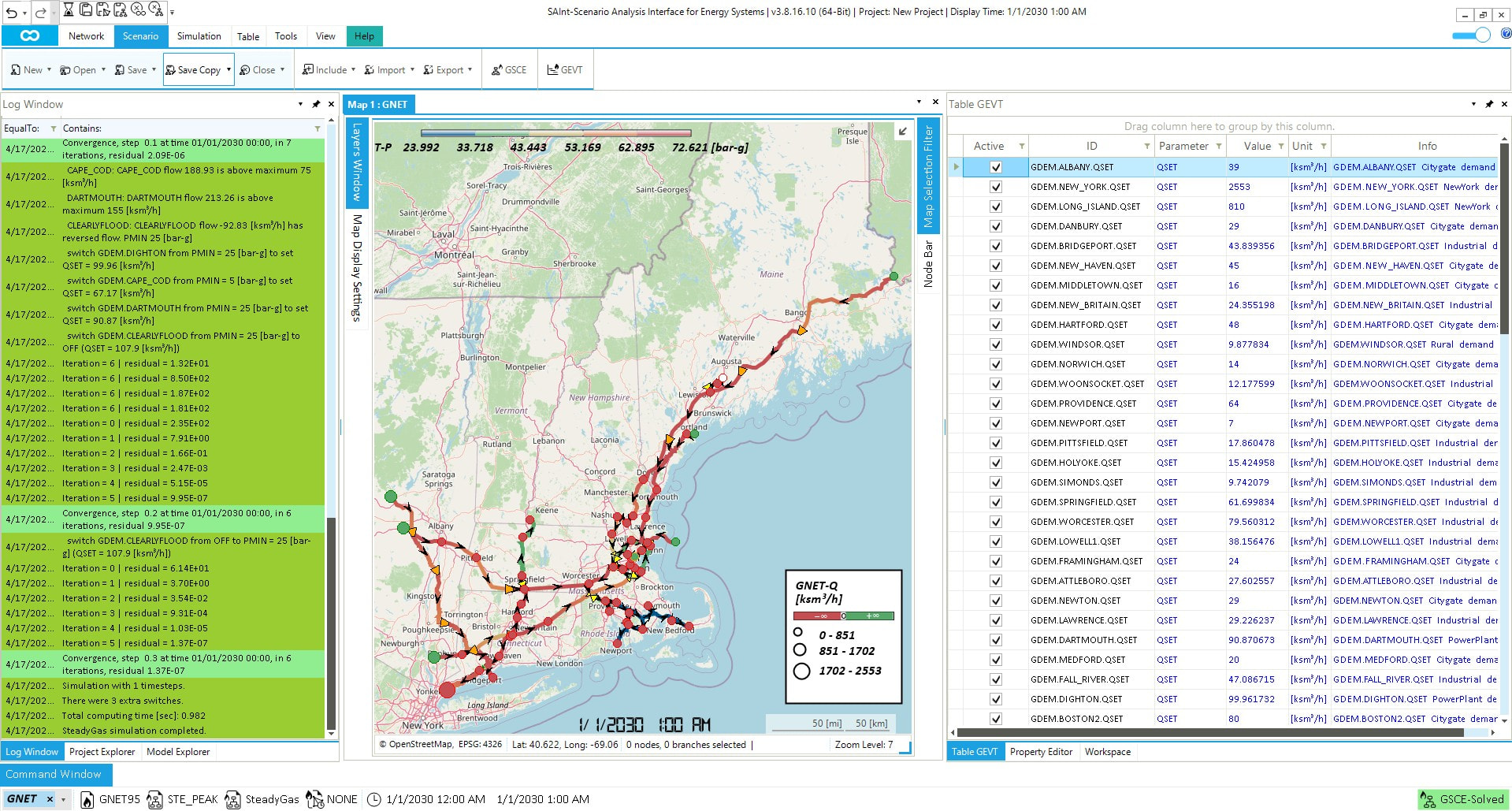
Figure 2: GNET95 branch pressure levels under design conditions
Flow and Volume Events
A total of 59 flow and volume events are defined:
- Flow set point (SAInt Event Parameter:
QSET): Defines injection or extraction rates (volumetric or energy terms). This scenario includes 50 extraction points (GDEM) and 5 injection points (GSUP, GSTR, LNG). In GSTR, a positive flow indicates the storage is in “discharge mode” and depletes its inventory to inject gas into the network (acting as a supply point). A negative flow indicates the storage is in “charging mode”, extracting gas from the network to replenish its inventory (acting as a demand point). - Initial storage inventory (SAInt Event Parameter:
INV): Sets the working gas inventory for GSTR or LNG. This scenario includes 3 events (1 for GSTR, 2 for LNG terminals). For LNG, INV represents the regasification storage at the terminal. - Bypass (SAInt Event Parameter:
BP): Configures the operation of a valve or compressor object as a passive branch, similar to a pipe or resistor. In this mode, the object does not influence pressure but allows flow to pass upstream or downstream. In this scenario, 1 event is defined for the GVA object that leads to the NEW_YORK demand hub. Similar to bypass, a non-return bypass (SAInt Event Parameter:NRBP) event operates the object passively, but with flow restricted to the direction defined by the valve or compressor object.
Temperature Events
A total of 10 temperature events are defined:
- Turn on temperature tracking (SAInt Event Parameter:
HTON): Activates temperature tracking at the network level. - Ambient temperature (SAInt Event Parameter:
TAMB): Adjusts ambient temperature at the network, subsystem, or branch level. This scenario includes 2 network events and another for the PROVIDENCE_BRANCH GSUB. - Supply temperature set point (SAInt Event Parameter:
TSET): Defines the temperature of the gas being injected to the network. This scenario includes 7 events across all GSUP, GSTR, and LNG objects.
STE_INI
The STE_INI scenario serves as the initial state for the dynamic DYN_FULL_YEAR scenario. The steady-state scenario is built as a snapshot of the gas infrastructure’s operation at the start of the year.
- Name: STE_INI
- Type: SteadyGas
Similar to STE_PEAK, this scenario includes three categories of events for pressure, flow, volume, and temperature. The pressure, volume, and temperature events remain the same. The difference between the scenarios lies in the flow setpoint, which is adjusted to match the demand, supply, and storage facility operational flows at the start of the year.
DYN_FULL_YEAR
This scenario is designed to simulate the operational conditions of the GNET95 transmission system, aimed at determining hydraulic behavior, inventory, linepack utilization, and end-user delivery over an entire year. It encompasses a full-year-round analysis covering all 8,760 hours to evaluate the system’s pressure levels and ensure end-user delivery constraints are respected across different seasons and operational conditions. It has the following properties:
- Name: DYN_FULL_YEAR
- Type: DynamicGas
- StartTime: January 1st, 2030
- EndTime: January 1st, 2031
- TimeStep: 60 min
- InitialState: STE_INI
Demand
The GNET95 network includes 50 GDEM objects, with a combined winter operational demand peak of 5.14 [Msm3/h] and an annual demand of 17,182 [Msm3], equivalent to 184 [TWh] of energy. Demand is split around 50/50 between the New York demand hub and the rest of the network.
As described in the Gas Demand section, three generic hourly demand profiles were developed to represent the seasonal, weekly, and daily variability of different end-user types: CITY_DEMAND_SHAPE, INDUS_DEMAND_SHAPE, and RURAL_DEMAND_SHAPE.In addition, five hourly demand profiles were created for generator off-take sites, classified as GFG_[GENERATOR]_DEMAND_SHAPE.
The profiles are linked to the GDEM objects, depending on the type of demand, using the flow set point (SAInt Event Parameter: QSET) scenario event. This event adjusts the QSET value of the GDEM object at each time step by scaling the demand shape profile according to the event value.
Supply
The GNET95 network includes four GSUPs and two LNG terminals, representing the supply points in the network. As described in the Gas Supply, LNG Terminals, and Underground Storage section, depending on the type of supply, they operate differently:
- National Cross-Boarder (SUP_CAN): The supply points WADDINGTON and SAINT_JOHN represent contractual flows between the Canadian and American border. The flow is adjusted weekly based on historical seasonal demand patterns. Each GSUP has a unique profile, which varies as a percentage of the maximum transfer volume at the interconnection. The profile is linked to the supplies using a flow set point (SAInt Event Parameter:
QSET) scenario event. This event adjusts the flow of the GSUP object at each time step by scaling the demand shape profile according to the event value. The SAINT_JOHN is isolated and requires a secondary pressure set point (SAInt Event Parameter:PSET) scenario event to adjust the pressure at the supply point if the downstream compressor station receives gas outside its typical operating range. This is implemented using a conditional event that adjusts the inlet pressure of the GCS_009 compressor station. - Interstate Cross-Boarder (SUP_US): The supply points SCHENECTADY and NEWBURGH respresent interconnection with the larger US gas infrastructure. The flow is used as a secondary supply to ensure system reliability, especially for the WESTERN_TRUCK, which delivers gas to the main demand hub. The GSUP operates using a pressure control event with a fixed pressure throughout the year.
- LNG Terminals (SUP_LNG): The LNG terminals STELLWAGEN and SOUTH_PORTLAND represent terminals that operate to provide the network with a constant flow. This is defined using the flow setpoint. The STELLWAGEN terminal uses conditional events to determine the flow, which is dependent on the gas extracted from the BOSTON_RING subsystem. During peak demand periods, the terminal will operate both supply trains, and during other periods, only a single train is used. Each terminal receives monthly vessels to meet its operational needs. The STELLWAGEN varies the vessel size to match its variable operation, while the SOUTH_PORTLAND has a fixed vessel size matching the fixed flow.
Storage
The GNET95 network includes an underground sotrage facility connected to the BOSTON_RING, the role of the facility is to help maintain the delivery pressure for the end user in the urban area. The storage can either extract and inject gas into or out of the network to help maintain pressure. The CHELSEA storage facility is operated using a set of pressure control set points (SAInt Event Parameter: PSET) scenario events. The primary event is used as a fixed reference point for typical operations. While the secondary event is triggered when the facility reaches max inventory, it slightly increases operational pressure to allow the storage to inject more gas into the network and deplete the inventory.
Results
After setting up a scenario with its specific settings and adding all the relevant profiles and events, it can then be simulated for analysis. The results of the scenario are stored in a solution file with the file extension *._sol (for example, *.gsol for gas network solutions).
The figures below show end-user demand in the New England Region, gas curtailment due to minimum delivery pressure requirements, and supply from different sources. It shows fluctuations in demand throughout the year, demonstrating how each gas supply source contributes to meeting demand. Table 5 provides the annual demand percentage for each sector.
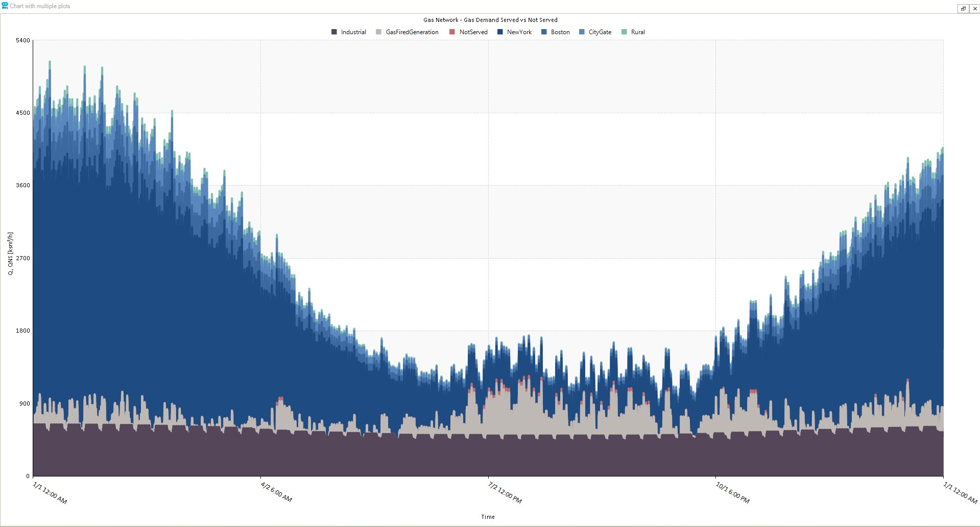
Figure 3: Annual gas demand served per gas group versus demand not served
TIP
The plot displayed above can be generated using the IronPython script titled “results_gas_demand.ipy,” which can be executed from the Script Editor within the SAInt GUI.
Table 5: Annual Gas Demand per Demand Group
| SAInt Group | Gas Demand Description | Annual Demand, [Msm3] | Percentage, [%] Total Demand |
Percentage, [%] Excluding New York Hub |
|---|---|---|---|---|
| NYC | New York City & Long Insland | 9,242 | 53.8 | - |
| BOS | Boston | 1,071 | 6.23 | 13.5 |
| CGS | Citygate Stations | 950 | 5.52 | 11.9 |
| RUR | Rural & Agricultural | 270 | 1.57 | 3.39 |
| IND | Industrial Facilities | 4,597 | 26.7 | 57.8 |
| GFG | Power Plants & Electric Production | 1,051 | 6.11 | 13.2 |
| GDEM.%.QNS | Total Demand Not Served | 11 | 0.07 | 0.14 |
DYN_GDNS_WEEK
The DYN_GDNS_WEEK scenario provides a focused, higher-resolution analysis of the week with the highest level of gas demand not served or gas curtailment in the DYN_FULL_YEAR scenario. To determine which week of the year this occurs, use the following prompt in the SAInt Command Window:
inttable(gsum('GDEM.%.QNS.[ksm3/h]'), '168[h]')
This prompt creates an integral table showing the total unmet demand across all gas demand objects in the network for each week of the DYN_FULL_YEAR scenario. The resulting table can then be used to identify the worst week, as shown below.
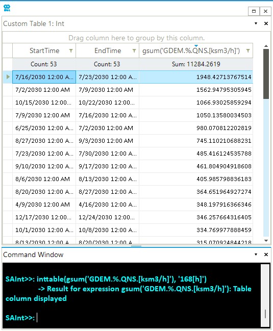
Figure 4: Using inttable to evaluate the week with the highest demand not served
Based on the results, we can determine that the week with the highest curtailment runs from July 16th to 23rd. A new DYN_GDNS_WEEK scenario will then be built using these dates. Before creating the new scenario, export the network’s condition at the start of that week. To do this use built-in display time function (time('7/16/2030 12:00 AM')). This command changes the time displayed in the SAInt Map Window. Check the displayed time at the bottom of the map to confirm it is correct. Once the correct time is set, export the network condition by navigating to:
Scenario tab > Export > Network State > Gas Network State (GCON)
This will create a condition file (*.gcon) in your network folder. Save this file as INI_GDNS.gcon.
NOTE
By default, SAInt interprets time using your computer’s local date and time format. If thetime()prompt returns an error or does not behave as expected, adjust the input format to match your computer’s DateTime settings and try again. For additional support, please post in the General section of the forum.
With the peak demand curtailment week identified and the condition file exported, create the new DYN_GDNS_WEEK scenario using the following properties:
- Name: DYN_GDNS_WEEK
- Type: DynamicGas
- StartTime: July 16th, 2030
- EndTime: July 23rd, 2030
- TimeStep: 5 min
- InitialState: INI_GDNS
As with DYN_FULL_YEAR, this scenario includes three categories of events: pressure, flow, volume, and temperature. The event values (SAInt Event Parameter: Value) and assigned profiles (SAInt Event Parameter: Profile) remain the same.
The main difference is that the event start times (SAInt Event Parameter: StartTime) must be shifted to align with the new scenario start. In contrast, the profile start times (SAInt Event Parameter: PrfStartTime) remain at the beginning of the year. In other words, the scenario window is shifted, but the original time-series sequencing is preserved. Additionally, any events that fall outside the new scenario time window must be removed. This may include, for example, vessel arrival events (SAInt Event Parameter: VESSEL) for LNG terminals.
Use the provided scenario profile and event template files to import the required data and execute the scenario. This scenario is intended to support the analysis of operational constraints and bottlenecks, as well as the evaluation of design alternatives and what-if scenarios.