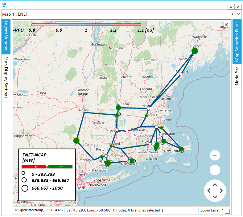
The ENET39 network is a modified version of the IEEE 39-bus Test System, representing the network of the New England region in the United States.
Download it here: ENET39 v24.9.20.zip (29.1 MB)
Disclaimer
The ENET39 dataset overlays a representation of a part of the United States with an existing power system. However, it is not a technically rigorous representation of this system. The names of nodes and generators are purely suggestive. Transmission line voltage ratings and capacities are set for illustrative purposes only.
The network layout over the New England area is roughly based on the layout depicted in Figure 2 of the cited source. Beyond this, no additional data from the referenced document was used in the creation of this dataset.
G. Tricarico, R. Wagle, M. Dicorato, G. Forte, F. Gonzalez-Longatt, and J. L. Rueda, “Zonal Day-Ahead Energy Market: A Modified Version of the IEEE 39-bus Test System,” in 2022 IEEE PES Innovative Smart Grid Technologies - Asia (ISGT Asia), Nov. 2022, pp. 86–90. doi: 10.1109/ISGTAsia54193.2022.10003588.
This model, developed by encoord GmbH for the Scenario Analysis Interface for Energy Systems (SAInt) planning software, is provided “as is” at no cost. encoord GmbH disclaims all responsibility for its use by others and makes no warranties, express or implied, regarding its quality, reliability, safety, or suitability. encoord GmbH will not be liable for any direct, indirect, or consequential damages related to its use.
Overview
The ENET39 network is a modified version of the IEEE 39-bus Test System, representing the network of the New England region in the United States. The network is on a 100 [MVA] base and the network voltage level is 20-345 [KV]. Table 1 below provides an overview of the components that form the network’s topology.
| SAInt Object Type | Representative Object | Count |
|---|---|---|
| ENO | Nodes (Buses) | 39 |
| LI | Electric Lines | 34 |
| TRF | Transformers | 12 |
The network is composed of 19 demands (SAInt Object Type: EDEM) with the peak power equal to 6.125 [GW]. Table 2 provides an overview of the generation fleet:
| SAInt Object Type | Generation Type | Capacity [GW] | Count |
|---|---|---|---|
| PV | Solar PV | 0.63 | 6 |
| WIND | Wind Onshore | 0.41 | 3 |
| FGEN | CCGT | 3.43 | 6 |
| FGEN | Coal | 2.0 | 2 |
| FGEN | Nuclear | 1.19 | 2 |
Developing the ENET39 Network: An Expansion of the IEEE 39-bus Test System
In SAInt, a network is a directed graph comprising of objects such as nodes, branches, and externals. These objects are interconnected and may be supplemented by auxiliary objects that represent or facilitate connections between them. Each network is characterized by its geometric, topological, relational, and static properties of all its objects.
The ENET39 network expands upon the foundational IEEE 39-bus Test System. The sections below explain the key network expansions.
Integrating Renewable Energy
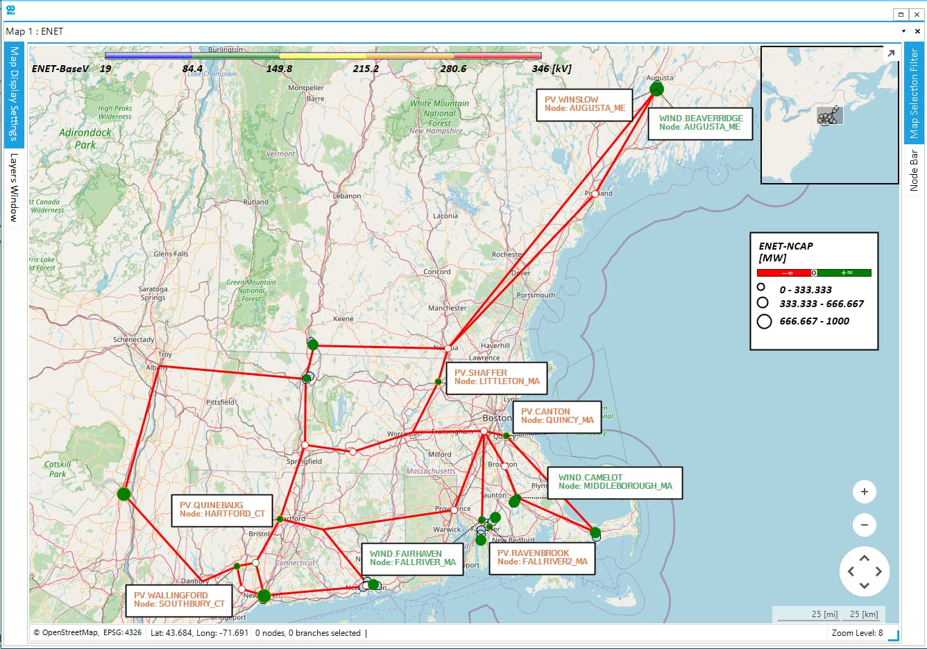
There are 10 generators in the original IEEE 39-bus Test System. In ENET39 network, three WIND and six PV plants are installed at different locations in the network. They are connected at the network voltage level, where the assumption that any requisite transformers to interconnect at this voltage are contained in the renewable generator object. Figure 2 below identifies the specific node locations of the WIND and PV plants:
| SAInt Object Type | Generator Name | RATEDS [MVA] | PMAXDEF [MW] | QMAXDEF [MVAr] | QMINDEF [MVAr] |
|---|---|---|---|---|---|
| PV | Wallingford | 200 | 180 | 40 | -40 |
| PV | Quinebaug | 150 | 135 | 30 | -30 |
| PV | Ravenbrook | 150 | 135 | 30 | -30 |
| PV | Canton | 100 | 90 | 20 | -20 |
| PV | Shaffer | 50 | 45 | 10 | -10 |
| PV | Winslow | 50 | 45 | 10 | -10 |
| WIND | Fairhaven | 200 | 180 | 40 | -40 |
| WIND | Camelot | 150 | 135 | 30 | -30 |
| WIND | Beaverridge | 100 | 90 | 20 | -20 |
where:
- RATEDS: Maximum apparent rated power capacity
- PMAXDEF: Default maximum active power capacity (i.e., nameplate installed capacity)
- QMAXDEF: Default maximum reactive power capacity
- QMINDEF: Default minimum reactive power capacity
Generator Operational and Cost Parameters
The original generators in the IEEE 39-bus Test System are modelled as fuel generators (SAInt Object Type: FGEN). Additional properties (listed below) for operational and cost parameters are included to facilitate market optimization modeling. The values for these properties are assigned based on the assumed generator type and size. These values are suggestive and intend to establish a reasonable representation generators operating in a power market.
Additional Operational Parameters
- PMINDEF: Default minimum stable generation
- MaxUp/DownRampDef: Default maximum up and down ramp rates
- MinUp/DownTimeDef: Default minimum up and down times
- Linear fuel consumption function:
- FC0: Constant fuel consumption coefficient
- FCI: Linear fuel consumption coefficient
- Linear heat rate function:
- HR0: Constant heat rate coefficient
- HR1: Linear heat rate coefficient
Additional Cost Parameters
- StartupPriceDef: Default start-up price
- VOMPriceDef: Default variable operational and maintenance cost
Note
All the PV and WIND generators are modeled with zero start-up and variable operational and maintenance costs.
Fuel Objects
In SAInt, each FGEN object has to be associated with a fuel object (SAInt Object Type: FUEL), which determines the fuel cost among other crucial emission factors. Table 3 below displays the FUEL objects included in the ENET39 network:
| Name | FuelPriceDef [$MMBTU] | CO2Emissions [g/MMBTU] | SO2Emissions [g/MMBTU] | NOXEmissions [g/MMBTU] |
|---|---|---|---|---|
| Uranium | 0.8 | 0 | 0 | 0 |
| Natural Gas | 4.5 | 53454 | 0.272 | 36.24 |
| Coal | 2.75 | 95130 | 40.82 | 36.29 |
where:
- FuelPriceDef: Default fuel price
- CO2Emissions: CO2 emission per fuel unit
- SO2Emissions: SO2 emission per fuel unit
- NOXEmissions: NOx emission per fuel unit
Ancillary Services
For the ENET39 network’s market optimization, one ancillary service (SAInt Object Type: ASVC) object named RESERVE_REQUIRMENT is included to represent an upward ramping reserve requirement. All Coal and CCGT generators within the ENET39 network contribute to this requirement via their corresponding ancillary service external (SAInt Object Type: ASVCX) objects.
Branch Capacities
In the ENET39 network, all electric lines (SAInt Object Type: LI) are standardized to include active power capacity of 700 [MW]. These lines are modelled to handle a maximum apparent power of 750 [MVA] and a maximum current magnitude of 1200 [A]. For the network transformers (SAInt Object Type: TRF), the capacity to transmit active power is higher - set at 1000 [MW] - with a maximum apparent power rating of 1200 [MVA].
Zero Sequence Parameters
To facilitate including the ENET39 network with other subtransmission/distribution networks in unbalanced AC power flow simulations, zero sequence parameters are defined based on the positive sequence parameters for all the LI objects. For TRF objects, only positive sequence parameters are applied, with all windings assumed to be in a Wye-Wye configuration. Additionally, it is assumed that the demand objects are balanced Wye loads and the generator objects are balanced Wye connected.
Zero sequence parameters, represented below with the subscript _0, are calculated based on the positive sequence parameters, indicated by subscript _1. Values for the positive sequence parameters come directly from the original IEEE 39-bus Test System.
- Resistance: R_0 = 3 \times R_1
- Reactance: X_0 = 3 \times X_1
- Susceptance: B_0 = \frac{B_1}{3}
Modeling Scenarios with ENET39
In SAInt, a scenario represents a specific case study applied to a network. A scenario is characterized by its type (e.g., SteadyACPF, SteadyUACPF, or DCUCOPF), a time window (start time, end time) and other time-dependent properties such as time step, time horizon, time look-ahead, and time step look-ahead. It may also include a set of events and profiles. An event denotes a change in settings, controls, or constraints of an object at a specific time during the scenario’s execution. A profile is a sequence of equidistant data points that includes information on how these data points are processed in terms of time step, interpolation, sampling, and periodicity. A profile can be assigned to an event to control the event’s value over time.
Tip
- The scenario profiles can be viewed through SAInt GUI by navigating to the Scenario Tab and selecting [EPRF] button, after loading the network and scenario files.
- To explore the list of events that are part of a scenario, navigate to the Scenario Tab and select [EEVT] after loading the corresponding network and scenario files.
A scenario allows for systematic and repeatable analysis of network behavior under varying conditions. For the ENET39 network, five scenarios have been developed, categorized into three scenario types:
- SteadyACPF (Steady-state AC power flow)
- DCUCOPF (Direct Current Unit Commitment Optimal Power Flow)
- QuasiDynamicACPF (Quasi-dynamic balanced AC power flow)
ACPF_IEEE39_BASE_RESULTS
This scenario is designed to validate the steady-state AC power flow simulation of the ENET39 network by comparing it to the power flow values from the IEEE 39-bus Test System .RAW file. The validation is performed by aligning the generation and demand configurations of the ENET39 with the settings in the IEEE 39-bus Test System. For instance, the additional WIND and PV generators in the ENET39 are configured to provide no contribution to both active and reactive power.
The scenario configures the ENET39 network to reproduce the results from the IEEE 39-bus Test System and has the following properties:
- Name: ACPF_IEEE39_BASE_RESULTS
- Type: SteadyACPF
There are three sets of events included in this scenario:
Active power set point (SAInt Event Parameter: PSET)
This scenario includes 38 active power set point (PSET) events: 10 for FGEN; 6 for PV; 3 for WIND; and 19 for EDEM objects. For FGEN, PV, and WIND generators, the events set the active power generation, while for EDEM objects the events set the active power consumption. For all PSET events, the event Value references the object’s PSETDEF property, which specifies the default active power set point.
Slack participation factor set point (SAInt Event Parameter: PFSET)
This scenario includes 10 slack participation factor set point (PFSET) events for the 10 FGEN objects. This event sets the slack contribution factor constraint for all the FGENs in the network by referencing the object’s PFSETDEF property, which specifies the default slack participation factor.
Voltage magnitude set point (SAInt Event Parameter: VMSET)
This scenario includes 10 voltage magnitude set point (VMSET) events for the 10 FGEN objects. These events set the voltage magnitude in per unit for all the FGENs in the network by referencing the object’s VMSETDEF property, which specifies the default voltage magnitude set point in per unit.
Tip
In this SteadyACPF scenario, the default property values already set the appropriate constraints, so adding these events isn’t necessary. However, if you need to change a constraint value, it’s best to do so using scenario events rather than altering the default property at network level. This approach ensures that changes are specific to the scenario and don’t unintentionally affect other scenarios that may not require the same adjustments.
The validation results of the voltage magnitude and angles are given in AC Power Flow Validation.
PCM_FULL_YEAR
This scenario is designed for the market optimization of the ENET39 transmission system, aimed at determining the economically optimal unit commitment and dispatch over an entire year. It encompasses a full year-round analysis, covering all 8,760 hours, to evaluate the system’s performance and economic efficiency throughout different seasons and operational conditions. It has the following properties:
- Name: PCM_FULL_YEAR
- Type: DCUCOPF
- StartTime: January 1st, 2023
- EndTime: January 1st, 2024
- TimeStep: 60 min
- TimeHorizon: 24 hrs
- TimeLookAhead: 24 hrs
- TimeStepLookAhead: 60 min
Demand
The ENET39 network includes 19 EDEM objects, with a combined peak power of 6125.4 [MW]. Seven hourly demand profiles are added to this scenario, each representing the demand shape of a different state in the region. These profiles are identified by state abbreviations such as NY_DEMAND_SHAPE.
The profiles are linked to the EDEM objects, using the active power set point (PSET) scenario event. This event adjusts the PSET value of the EDEM object at each time step by scaling the demand shape profile according to the event Value, which is defined by the PSETDEF property of the object. The PSETDEF property specifies the default active power set point, in this case representing the peak power consumption.
Note
The SAInt property “PSETPRCDEF” for EDEM objects defines the “price of load shedding”, “value of lost load”, etc., which defines how much the objective function will increase for each 1 [MW] of demand that is not met with generation. A value of 100,000 [$/MWh] is assigned to each EDEM object in the ENET39 network.
Renewable Generation
The ENET39 network includes six PV and three WIND generators representing the renewable generation in the network. Nine hourly normalized profiles are added into the PCM_FULL_YEAR scenario, each representing the generation of the PV and WIND objects. These profiles are identified by unique names, such as PV_RAVENBROOK_PSET_PU.
The generation profiles are linked to the PV and WIND objects, using the PSET scenario event. This event adjusts the PSET value of the PV or WIND object at each time step by scaling the normalized profile according to the event Value, which is defined by the PMAXDEF property of the object. The PMAXDEF property specifies the default maximum active power, in this case, representing the installed capacity.
Ancillary Service Requirement and Contribution
In this scenario, the ancillary service requirement and contribution are modelled using the following scenario events.
-
Requirement: The minimum requirement for the ASVC object RESERVE_REQUIREMENT is modelled using a MinVal event. This event sets the requirement to be equal to 3% of the total network demand at each timestep.
-
Contribution: Contributions from fuel generators to the ancillary service are defined using the MaxVal event of the ASVCX object. This event sets the contribution to be equal to ten times the generator’s maximum upward ramp rate at each time step.
Note
The SAInt property “MinValPriceDef” for ASVC objects defines the “price of reserve requirement shedding”, “value of lost reserves”, etc., which defines how much the objective function will increase for each 1 [MW] of reserves that is not met with generation. A value of 10,000 [$/MW] is assigned to the “RESERVE_REQUIREMENT” ASVC object.
Generator Maintenance and Must-Run Schedules
In this scenario, the generator maintenance and must-run requirements are modelled using scenario events.
-
Maintenance Outages: These are planned periods when generators are taken offline for maintenance. These are modelled using the paired “OFF” and “ONOFF” events. An “OFF” event marks the generator as temporarily non-operational, while an “ONOFF” event indicates a transition point where the commitment status of the generator can be set according to the optimal system oepration determined by the solver.
-
Must-Run Events: “ON” events are included for nuclear generators to ensure they remain operational. Note that events marking the end of maintenance outages for nuclear generators are “ON” events rather than “ONOFF”.
Results
After setting up a scenario with its specific settings and adding all the relevant profiles and events, it can then be simulated for analysis. The results of the scenario are stored in a solution file, which uses the file extension *._sol (for example, *.esol for solutions pertaining to electric networks).
Figure 3 shows the generation dispatch by generation type from multiple sources such as NUCLEAR, COAL, CCGT, WIND and PV, along with the renewable curtailments. It shows the fluctuations in generation for the whole year, demonstrating how each energy source contributes to meeting the demand. Table 4 alongside provides the annual percentage contributions of these energy sources.
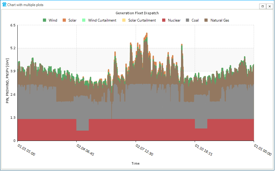
Tip
The plot displayed above can be generated using the IronPython script titled “results_pcm_full_year.ipy,” which can be executed from the Script Editor within the SAInt GUI.
Table 4: Annual Generation Mix by Generation Type
| Generation Type | Contribution [%] |
|---|---|
| Nuclear | 33.8 |
| Coal | 34.6 |
| CCGT | 23.5 |
| WIND | 3.9 |
| PV | 4.2 |
PCM_MIN_NET_DEMAND_WEEK
This scenario is a subset of the PCM_FULL_YEAR scenario aimed at determining the economically optimal dispatch for the minimum net demand week. It encompasses a full week analysis, covering 168 hours. It has the following properties:
- Name: PCM_MIN_NET_DEMAND_WEEK
- Type: DCUCOPF
- StartTime: May, 23rd, 2023
- EndTime: May 30th, 2023
- TimeStep: 60 min
- TimeHorizon: 24 hrs
- TimeLookAhead: 24 hrs
- TimeStepLookAhead: 60 min
The PCM_MIN_NET_DEMAND_WEEK scenario contains the same set of events and profiles as the PCM_FULL_YEAR with the updated event “StartTime” and “PrfStartTime”.
Figure 4 below offers insights into the operation of the network during the period of minimal net demand. It shows the generation fleet dispatch along with system demand over the minimum net demand week.
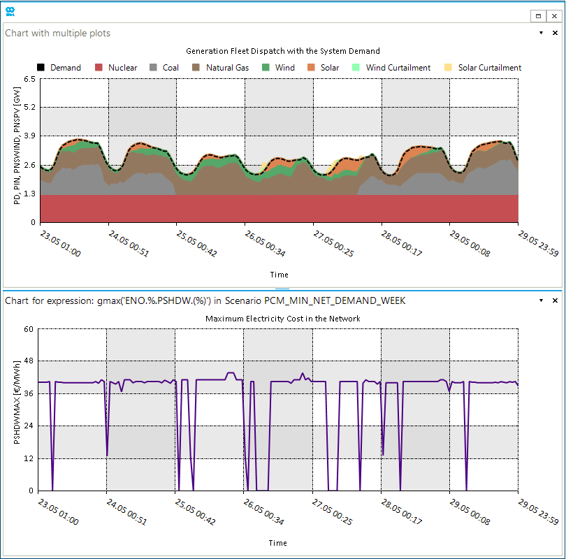
Tip
The plot displayed above can be generated using the IronPython script titled “results_pcm_min_net_week.ipy,” which can be executed from the Script Editor within the SAInt GUI.
PCM_PEAK_DEMAND_WEEK
This scenario is a subset of the PCM_FULL_YEAR scenario aimed at determining the economically optimal dispatch for the peak demand week. It encompasses a full week analysis, covering 168 hours. It has the following properties:
- Name: PCM_PEAK_DEMAND_WEEK
- Type: DCUCOPF
- StartTime: July, 16th, 2023
- EndTime: July 23rd, 2023
- TimeStep: 60 min
- TimeHorizon: 24 hrs
- TimeLookAhead: 24 hrs
- TimeStepLookAhead: 60 min
The PCM_PEAK_DEMAND_WEEK scenario contains the same set of events and profiles as the PCM_FULL_YEAR with the updated event “StartTime” and “PrfStartTime”.
Results
Figure 5 below offers insights into the operation of the network during the periods of peak demand. It shows the generation fleet dispatch along with system demand over the peak demand week.
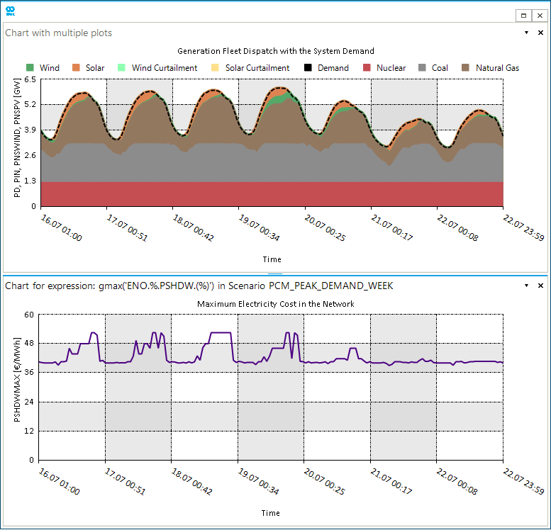
Tip
The plot displayed above can be generated using the IronPython script titled “results_pcm_peak_demand_week.ipy,” which can be executed from the Script Editor within the SAInt GUI.
ACPF_PEAK_DEMAND_WEEK
This scenario is designed for techno-economic analysis of the ENET39 transmission system over the peak demand week. It is aimed for understanding the reliabilty concerns during the week of peak demand using the optimal dispacth from the “PCM_PEAK_DEMAND_WEEK” scenario. It encompasses a full week analysis, covering 168 hours. It has the following properties:
- Name: ACPF_PEAK_DEMAND_WEEK
- Type: QuasiDynamicACPF
- StartTime: May, 23rd, 2023
- EndTime: May 30th, 2023
- TimeStep: 60 min
Demand
In this scenario, 19 hourly consumption profiles are added, each representing the consumption of the EDEM object, taken from the inputs of the PCM_PEAK_DEMAND_WEEK scenario. These profiles are identified by unique names, such as EDEM_HOLYOKE_DEMAND_PSET.
The profiles are linked to the EDEM objects, using the PSET scenario event. This event adjusts the PSET value of the EDEM object at each time step using the hourly consumption profile.
Generator Dispatch
In this scenario, the hourly dispatch profiles of all the generators are added. These profiles represent the least cost optimal dispatch of each generator from the solution of the PCM_PEAK_DEMAND_WEEK scenario. They are identified by unique names, such as, FGEN_SIMONDS_PSET.
The profiles are linked to the generator objects, using the PSET scenario event. This event adjusts the PSET value of the generator object at each time step using the hourly dispatch profile.
Note
The additional “ON” and “OFF” events for the FGEN objects are modelled to represent the unit commitment from the solution of the PCM_PEAK_DEMAND_WEEK scenario.
Results
For this scenario, let’s examine the operation of the WESTBROOK generator connected to the AUGUSTA2 node. Figure 6 below shows the operation of WESTBROOK and the corresponding voltage magnitude and angle at AUGUSTA2. Observations reveal a significant spike in voltage magnitude at the node whenever the generator goes offline, as part of the unit commitment under the PCM_PEAK_DEMAND_WEEK scenario. This spike occurs because, during periods of low demand, the network experiences excess reactive power and with the generator offline, the reactive power support drops to zero at this node.
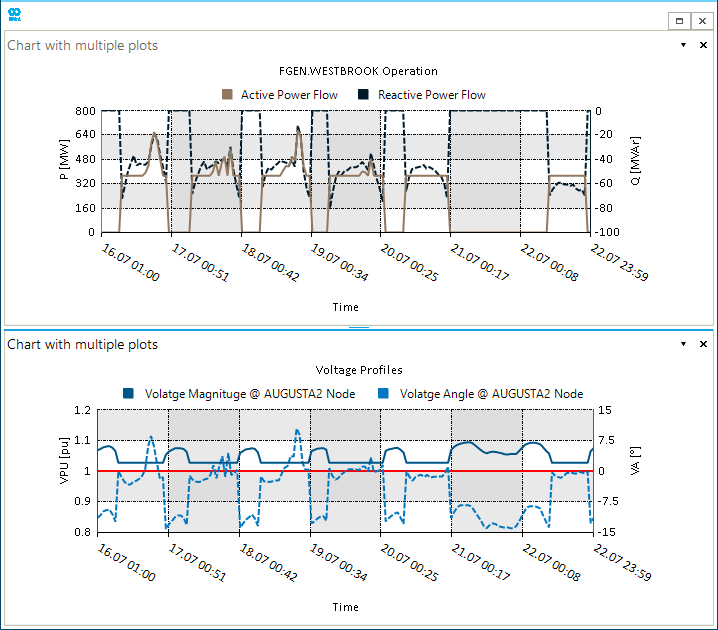
Tip
The plot displayed above can be generated using the IronPython script titled “results_acpf_peak_demand_week.ipy,” which can be executed from the Script Editor within the SAInt GUI.
AC Power Flow Validation
The included SAInt scenario ACPF_IEEE39_BASE_RESULTS configures the network to reproduce the IEEE 39 bus system response. The AC power flow validation is conducted by aligning the generation and demand configurations of the ENET39 network with the dispatch settings of the IEEE 39-Bus System. This alignment allows us to verify the network’s voltage magnitudes and angles by comparing them to the power flow values from PSS/E’s raw files, as shown in Table 5.
Table 5: Voltage magnitude and angles comparison
| Nodes | VPU [pu] | PSS/E_VPU [pu] | VA [°] | PSS/E_VA [°] |
|---|---|---|---|---|
| ALBANY_NY | 1.049 | 1.049 | -8.369 | -8.368 |
| GREENFIELD_MA | 1.052 | 1.052 | -5.772 | -5.772 |
| HOLYOKE_MA | 1.036 | 1.036 | -8.608 | -8.608 |
| HARTFORD_CT | 1.017 | 1.017 | -9.512 | -9.512 |
| PROSPECT_CT | 1.014 | 1.014 | -8.432 | -8.432 |
| NEWHAVEN_CT | 1.011 | 1.011 | -7.734 | -7.734 |
| ANSONIA_CT | 1.002 | 1.002 | -9.907 | -9.907 |
| SOUTHBURY_CT | 1.002 | 1.002 | -10.403 | -10.403 |
| DANBURY_CT | 1.031 | 1.031 | -10.165 | -10.165 |
| GROTON_CT | 1.021 | 1.021 | -5.306 | -5.306 |
| NEWLONDON_CT | 1.017 | 1.017 | -6.132 | -6.132 |
| NEWLONDON2_CT | 1.005 | 1.005 | -6.118 | -6.117 |
| GROTON2_CT | 1.02 | 1.02 | -5.999 | -5.999 |
| MARLBOROUGH_CT | 1.02 | 1.02 | -7.61 | -7.61 |
| PROVIDENCE_RI | 1.02 | 1.02 | -7.844 | -7.844 |
| BOSTON_MA | 1.035 | 1.035 | -6.374 | -6.374 |
| WORCESTER_MA | 1.038 | 1.038 | -7.421 | -7.421 |
| BRIMFIELD_MA | 1.036 | 1.036 | -8.299 | -8.299 |
| FALLRIVER_MA | 1.051 | 1.051 | -1.221 | -1.221 |
| FALLRIVER2_MA | 0.992 | 0.992 | -2.21 | -2.21 |
| BROCKTON_MA | 1.034 | 1.034 | -4.079 | -4.08 |
| MIDDLEBOROUGH_MA | 1.051 | 1.051 | 0.252 | 0.252 |
| HYANNIS_MA | 1.046 | 1.046 | -0.018 | -0.018 |
| QUINCY_MA | 1.041 | 1.041 | -6.294 | -6.294 |
| BRATTLEBORO_VT | 1.06 | 1.06 | -4.379 | -4.379 |
| NASHUA_NH | 1.055 | 1.055 | -5.594 | -5.594 |
| LITTLETON_MA | 1.041 | 1.041 | -7.581 | -7.581 |
| PORTLAND_ME | 1.052 | 1.052 | -2.091 | -2.091 |
| AUGUSTA_ME | 1.051 | 1.051 | 0.662 | 0.662 |
| TURNERSFALLS_MA | 1.048 | 1.048 | -3.36 | -3.36 |
| NEWHAVEN2_CT | 0.982 | 0.982 | 0 | 0 |
| MYSTIC_CT | 0.983 | 0.983 | 2.658 | 2.658 |
| FALLRIVER4_MA | 0.997 | 0.997 | 3.995 | 3.995 |
| FALLRIVER3_MA | 1.012 | 1.012 | 2.981 | 2.981 |
| MIDDLEBOROUGH2_MA | 1.049 | 1.049 | 5.208 | 5.208 |
| HYANNIS2_MA | 1.064 | 1.064 | 7.821 | 7.821 |
| BRATTLEBORO2_VT | 1.028 | 1.028 | 2.393 | 2.393 |
| AUGUSTA2_ME | 1.027 | 1.027 | 7.716 | 7.716 |
| KINGSTON_NY | 1.03 | 1.03 | -9.935 | -9.935 |
Note
The positive sequence resistance values in per unit (RRDEF) were adjusted from 0 to more realistic values, for the followiing transformers:
- GREENFIELD_MA_TO_TURNERSFALLS_MA
- NEWHAVEN_CT_TO_NEWHAVEN2_CT
- GROTON_CT_TO_MYSTIC_CT
- MIDDLEBOROUGH_MA_TO_MIDDLEBOROUGH2_MA
To reproduce the results shown in Table 5, reset the RRDEF values back to 0.